SOL 200 Web App
Installation Guide
Contents
- Preface
- Connected Clients
- What is design optimization?
- Description of MSC Nastran Design Sensitivity and Optimization
- SOL 200 Web App
- Apps
- Tutorials
- Optimization Basics
- Size Optimization Tutorials
- Topology, Topometry and Topography Tutorials
- Advanced Tutorials
- Miscellaneous Tutorials
- Machine Learning Tutorials
- Beams Tutorials
- Composite Laminate Optimization Tutorials
- Shape Optimization Tutorials
- Post-processor Tutorials
- Uncertainty Quantification
- Optimization Under Uncertainty
- Guidance on Configuring a Single Scalar Objective
- Frequently Asked Questions
- Uploading BDF Files
- Downloading Files and Executing MSC Nastran
- Optimization Types
- Supported Capabilities
Preface
About this Document
The SOL 200 Web App, web app for short, is a tool that facilitates the use of MSC Nastran's optimization capability available in solution sequence 200 (SOL 200). The purpose of this document is to detail information regarding fundamentals of optimization, what the web app is used for, learning resources, and installation details.
Technical Support
Users located in the country of Japan are encouraged to contact the MSC Software Support Team at the following email address: support.jp@mscsoftware.com.
All other users are to contact The Engineering Lab, christian@the-engineering-lab.com.
Training and Online Resources
The Tutorials section of this guide includes over 25 tutorials detailing the use of the web app and MSC Nastran SOL 200. PDF tutorials are available, and video tutorials are only available on YouTube.
Version
SOL 200 Web App Version 9.0.0 - 20260403_0800 Dev
Version Highlights
V8.5.0
| New Capabilities and Descriptions | Image of New Capability | ||||||||||||||||||||||||||||||||||||||||||||||||||
|---|---|---|---|---|---|---|---|---|---|---|---|---|---|---|---|---|---|---|---|---|---|---|---|---|---|---|---|---|---|---|---|---|---|---|---|---|---|---|---|---|---|---|---|---|---|---|---|---|---|---|---|
|
Uncertainty Quantification and Optimization Under Uncertainty
Before: Prior releases of the web app did not support uncertainty quantification or optimization under uncertainty. Uncertainty quantification (UQ) is the process of evaluating the uncertainty of inputs and outputs of a function, simulation model or physical system. Forward uncertainty quantification is the process of determining statistical quantities of outputs, or responses, when the inputs are uncertain. For example, a cantilever beam when mass produced will rarely yield beams with identical beam cross sections and identical performance. The variability of the beam cross sections will produce beams with a range of probable outputs, e.g. stress, displacement, etc. A goal of uncertainty quantification may be to determine the probability of failure, or the probability of manufactured beams exceeding the yield strength of the material when deviations in beam cross sections are taken into account. A second goal may be to automatically optimize the structural or mechanical system when considering constraints on probability of failure or to obtain a robust design. Optimization under uncertainty (OUU) may be employed to satisfy the secondary goal. After: This release now supports uncertainty quantification and optimization under uncertainty of MSC Nastran models. A UQ or OUU may be configured in the Machine Learning web app. Uncertain variables and responses may be selected and configured. Uncertain variables may be configured with one of the following distributions: normal uncertain, lognormal uncertain, uniform uncertain or continuous. Responses available in the MSC Nastran H5 file may be selected as uncertain responses. Typical outputs of UQ include mean, standard deviation, confidence intervals of mean and standard deviation, probability density function values (PDF), cumulative distribution function values (CDF) and complementary cumulative distribution function values (CCDF). The following UQ methods are supported.
OUU may also be configured. A reliability based design optimization (RBDO) may be configured by constraining probabilities of failure or reliability indices. A robust design optimization (RDO) may be configured by defining an objective that minimizes the sum of mean and three standard deviations of one or more responses. The following OUU approaches are supported.
One significant benefit of these new UQ and OUU capabilities is that no scripting is required. The web app utilizes Dakota to perform the uncertainty quantification or optimization under uncertainty. Dakota is one of the most sophisticated toolkits available for UQ and OUU. Dakota is open source and is developed by Sandia National Laboratories. This new capability is featured in the tutorials found in sections Uncertainty Quantification and Optimization Under Uncertainty. |

The distribution, mean and standard deviation are configured for uncertain variables. 
The results of a UQ are displayed and include the mean, standard deviation, confidence intervals and PDF, CDF or CCDF values for each response. 
A UQ method and OUU approach is selected in the web app. 
The results of an OUU are displayed. Summary tables are listed for the reliability constraints. The change of the robust design objective may be inspected. |
Version Highlights
V8.0.0
| New Capabilities and Descriptions | Image of New Capability |
|---|---|
|
Post-processor Web App
Before: Visualizing MSC Nastran results/responses is a critical step towards improving the performance of a mechanical or structural design. MSC Nastran supports a wide range of responses for 3D, 2D, 1D and 0D elements. Many post-processors are capable of displaying responses for 3D and 2D elements, but have limited support for responses of 1D and 0D elements. In other scenarios, post-processors display results only for the linear solution sequences, such as SOL 101 and 103, but do not support results from other solution sequences, such as the nonlinear analysis solution sequence SOL 400. Visualizing MSC Nastran results also requires the differentiation of domains of the results. Many of the MSC Nastran responses originate and are attributed with a different domain. Examples of domains include subcase number, time step, design cycle number and module number. Post-processors must be able to differentiate results from different domains, but many post-processors lack support for all possible domains. As an example, consider an optimization with MSC Nastran SOL 200. The responses will be attributed with a subcase number and design cycle number. Some post-processors support differentiation by subcase number, but not design cycle number. If the post-processor does not support differentiation for all domains, results within the post-processor will be misidentified. Many post-processors exist in the CAE market with the limitations mentioned in this section. After: This release includes a new Post-processor web app for MSC Nastran results. The goal of the Post-processor web app is to support visualization of results for 3D, 2D, 1D and 0D element types and support differentiation of domains. With the Post-processor web app, interpretation of MSC Nastran results is expected to be more practical and will aid in optimizing MSC Nastran models. Only the H5 results file is supported. The Post-processor web app is accessed within the Viewer. The Beams Viewer is no longer a separate web app and has been merged into the Post-processor web app. This new capability is featured in the tutorials found in the Post-processor Tutorials section. |
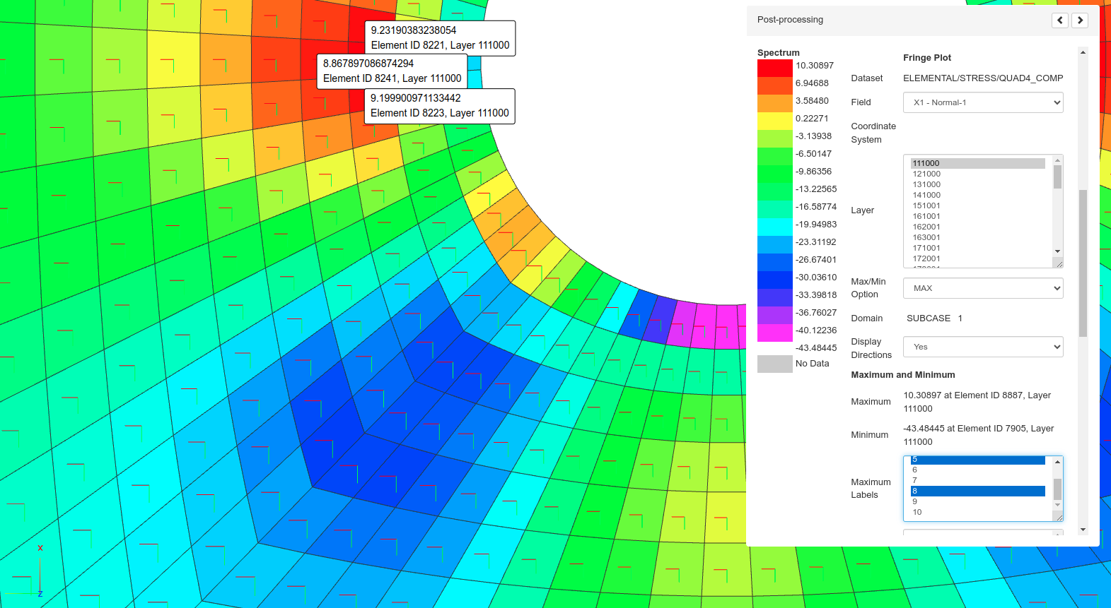
The Post-processor web app is used to display composite ply failure indices for GPLY 111000, maximum and minimum response labels, and direction of the ply. 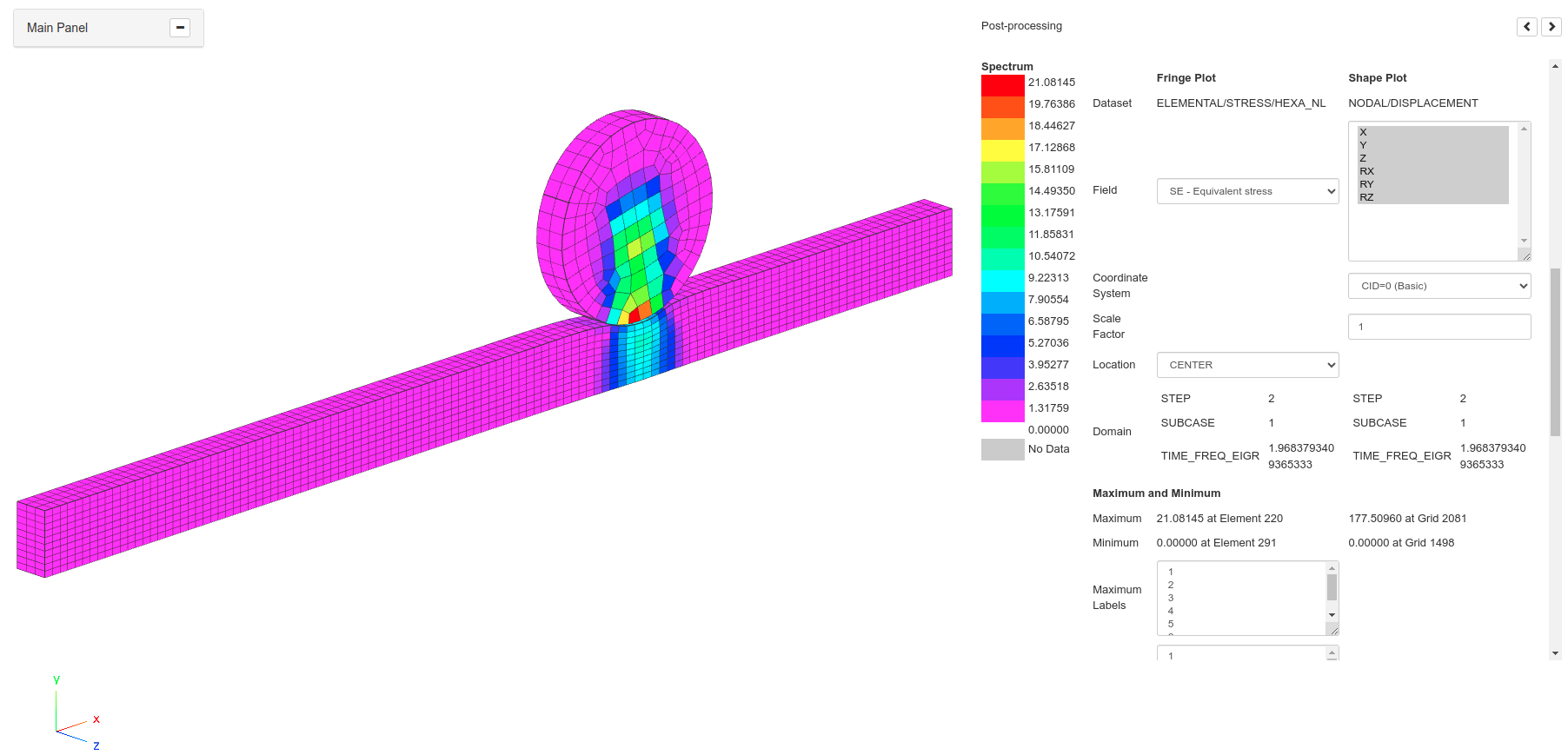
The Post-processor web app is used to display the results of a nonlinear analysis with MSC Nastran SOL 400. 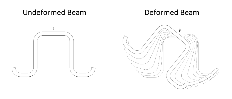
MSC Nastran outputs translations and rotations. The Post-processor web app displays deformed shapes by taking into account both translations and rotations. The rotations are displayed for 1D elements by showing twisting along the beam's length. |
|
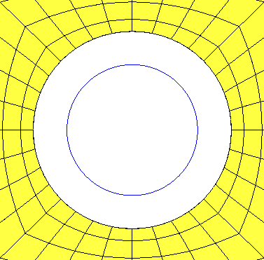
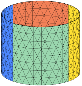
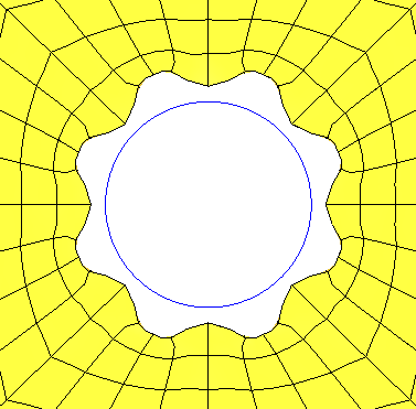
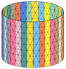
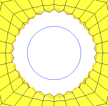
Support for symmetry constraints in a topometry optimization
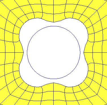
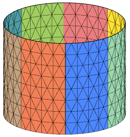
Before: Topometry optimization often yields results that are unsymmetrical. MSC Nastran 2024.1 now supports both mirror and cyclic symmetry constraints for topometry optimization. Obtaining symmetric results is now possible. To use symmetry constraints, the SYM keyword must be specified on the TOMVAR entry. After: The SYM keyword is now supported. A topometry optimization may be configured with mirror or cyclic symmetry constraints. This new capability is featured in the tutorial titled MSC Nastran Topometry Optimization with Symmetry Constraints. |
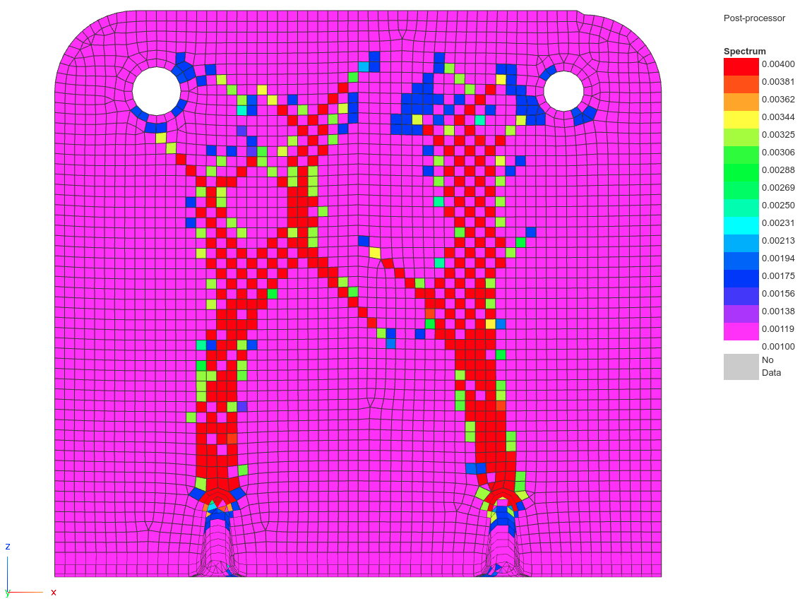
The results of a standard topometry optimization yields unsymmetrical results. 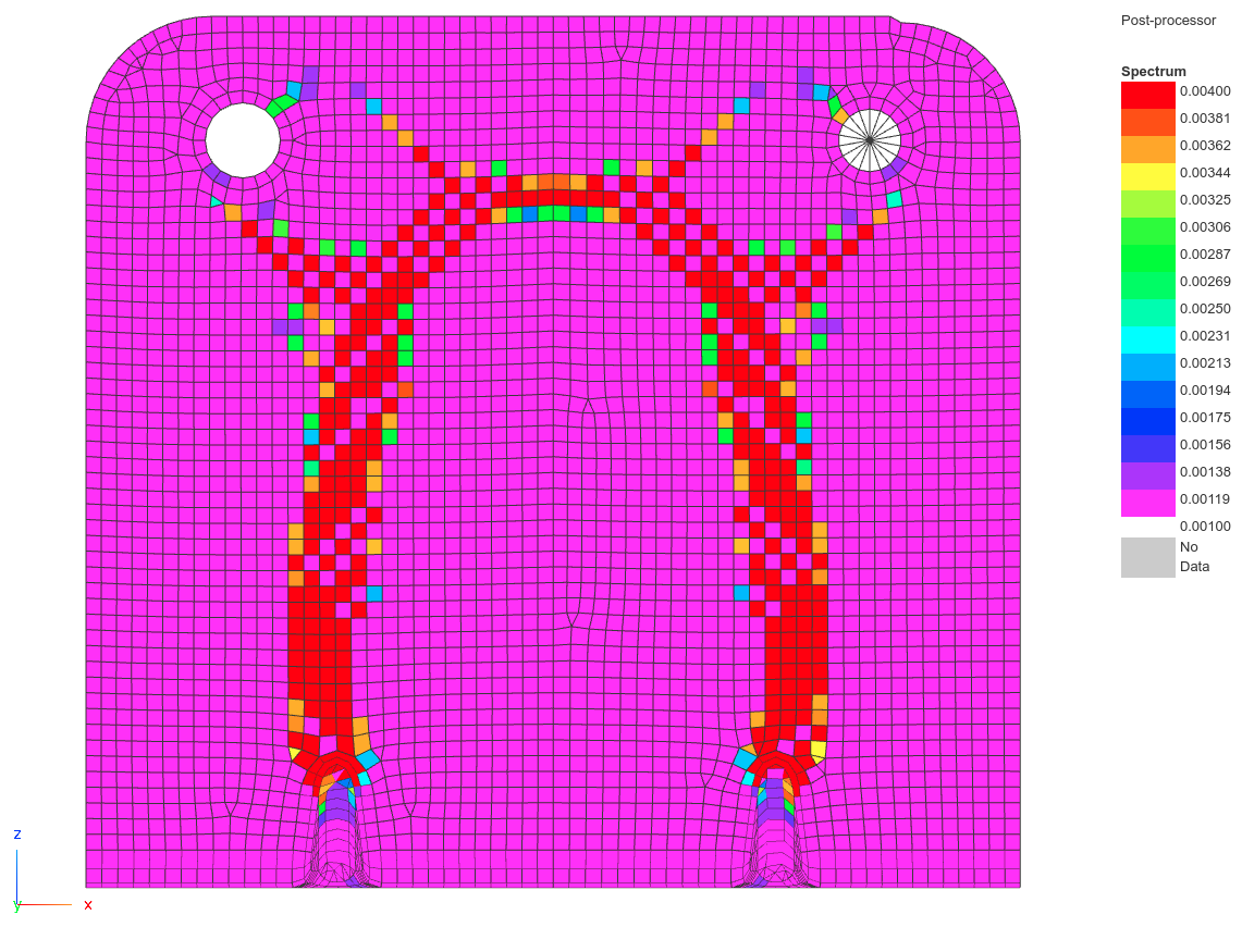
The results of a topometry optimization with mirror symmetry constraints yields symmetric results. |
V7.5.0
| New Capabilities and Descriptions | Image of New Capability | ||||||||||||||||||||
|---|---|---|---|---|---|---|---|---|---|---|---|---|---|---|---|---|---|---|---|---|---|
|
Dynamic Loads
Before: The RLOAD1 and RLOAD2 bulk data entries are used to define dynamic loads dependent on frequency. For simple dynamic loads, the bulk data entries RLOAD1 and RLOAD2 are defined. For more complex dynamic loads, the following entries may be defined: RLOAD1, RLOAD2, TABLED1, TABLED2, TABLED3, TABLED4, DELAY or DPHASE. Traditionally, the process of defining these entries is a trial and error process involving the following steps.
During this traditional procedure, an XY plot of the dynamic load is only visible in the final step. For steps 1, 2 and 3, the dynamic load is not immediately visible, which makes defining the dynamic load difficult. After: A new Dynamic Loads web app has been developed that is used to define dynamic loads. This web app defines the following entries: RLOAD1, RLOAD2, TABLED1, TABLED2, TABLED3, TABLED4, DELAY, DPHASE and DLOAD. As the dynamic load is configured, the web app automatically generates an XY plot of the applied load. For example, adjusting the delay or phase angle immediately updates a plot of the dynamic load. To be fully confident the applied load has been defined as intended, a test MSC Nastran run may be performed and the nastran generated dynamic loading may be inspected. Also, a Subcases section allows assigning dynamic loads to different subcases and with different scale factors. Internally, the web app automatically generates DLOAD entries and updates the DLOAD commands in the case control section. This new capability is featured in the tutorial titled Creation of Dynamic Loads via RLOAD1 or RLOAD2 Entries. |
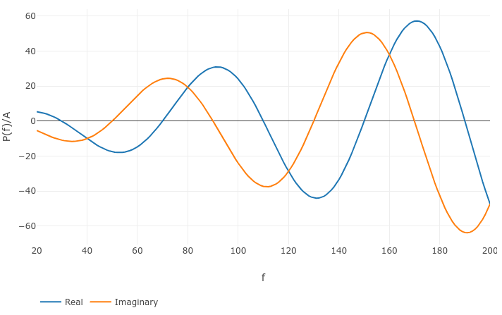
The temporal distribution of dynamic load for an RLOAD1 entry is generated by the Dynamic Loads web app. An option to switch to an RLOAD2 entry is available. 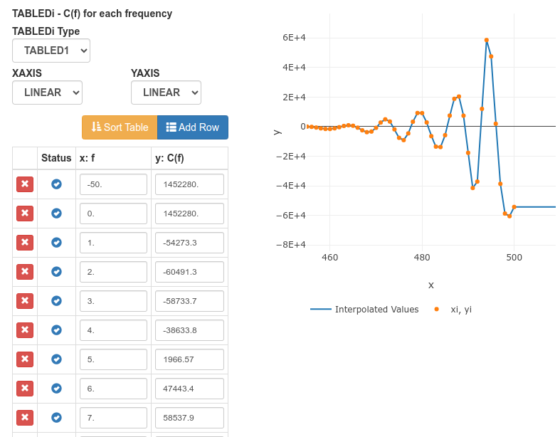
A preview of the TABLED1 interpolated values is generated by the Dynamic Loads web app. 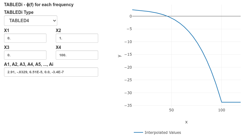
A preview of the TABLED4 interpolated values is generated by the Dynamic Loads web app. 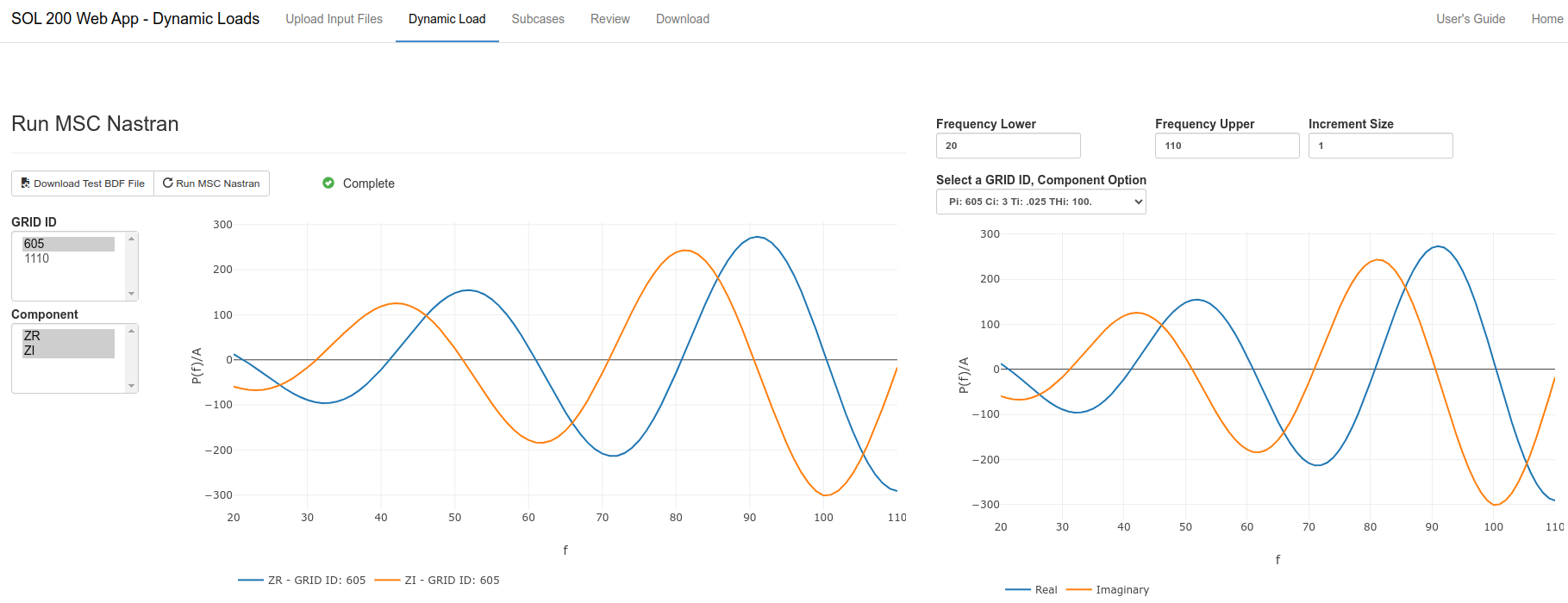
Right: The dynamic load generated by the web app is displayed. Left: The dynamic load generated by an MSC Nastran test run is displayed. The web app generates a preview of the dynamic load and an MSC Nastran test run confirm the dynamic load has been defined as intended. |
||||||||||||||||||||
|
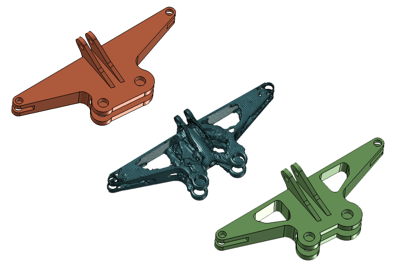
Shape Optimization for Conceptual Design of 3D Element Models
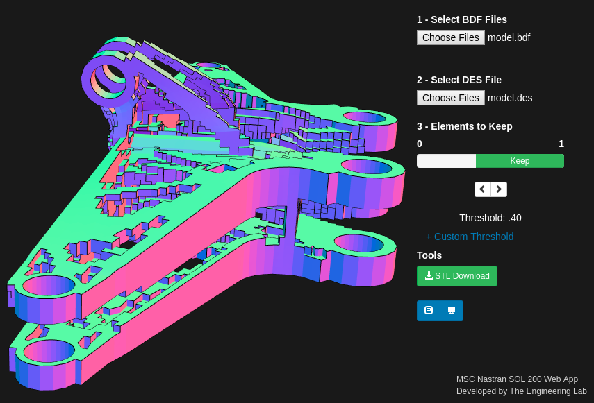
Before: One critical step in performing shape optimization of finite element models is prescribing the allowable movement of nodes in the model. When the model has thousands or millions of nodes, this becomes a tedious process. Methods currently exist to make the process simpler, and in this release, a new user interface is introduced to enhance a specific shape optimization method. The boundary shape method, either via geometry boundary shape or analytic boundary shapes, involves specifying the allowable node changes on the boundaries of the mesh, which are then interpolated to the interior nodes. The allowable node changes on the boundaries and interior constitute the shape basis vectors. Users can control the number of parameters involved in this type of shape optimization. For example, consider a geometric hole. Either each node along the circumference of the hole is allowed to change independently or all the nodes change together in the radial direction. The boundary shape method ranges between moderate to high difficulty. After: A new user interface to shape optimization is available in the Viewer web app. Users may select groups of nodes on the boundary that will either expand or contract together. Internally, the web application will manage all the necessary case control commands and bulk data entries necessary to perform the shape optimization. The web app adopts the auxiliary boundary shapes method. For each design region, or group of nodes on the boundary, an auxiliary model involves applying a pressure load (PLOAD4) or a temperature load (TEMPD) to expand or contract the selected element faces. The new interface also includes preview functionality. The shape changes may be previewed and users may specify ideal bounds on the shape variables to avoid mesh distortions. Since this strategy to shape optimization is convenient to configure but yields shapes of varying smoothness, it is recommended this shape optimization strategy be used to develop conceptual designs. This new interface is limited to finite element models composed of 3D elements: CHEXA, CTETRA, CPENTA or CPYRAM elements. This new interface does not support shape optimization for 1D or 2D elements. Only auxiliary models configured by this web app are supported. This new capability is featured in the tutorials found in the Shape Optimization Tutorials section. |
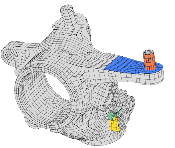
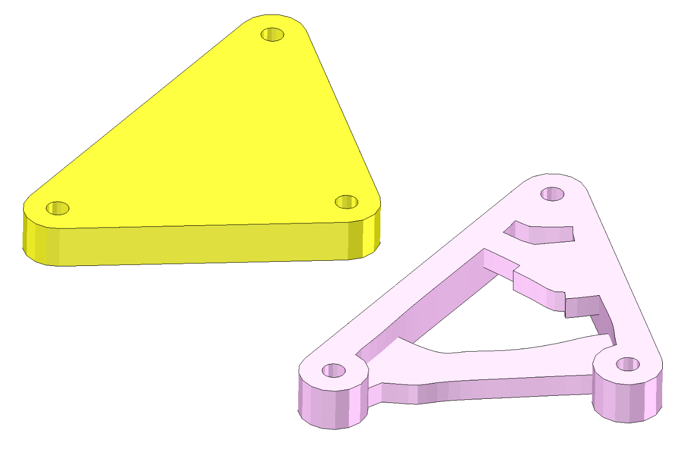
Example: Shape optimization of an automotive steering knuckle. 
Shape optimization animation of a steering knuckle. 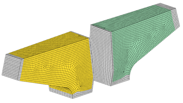
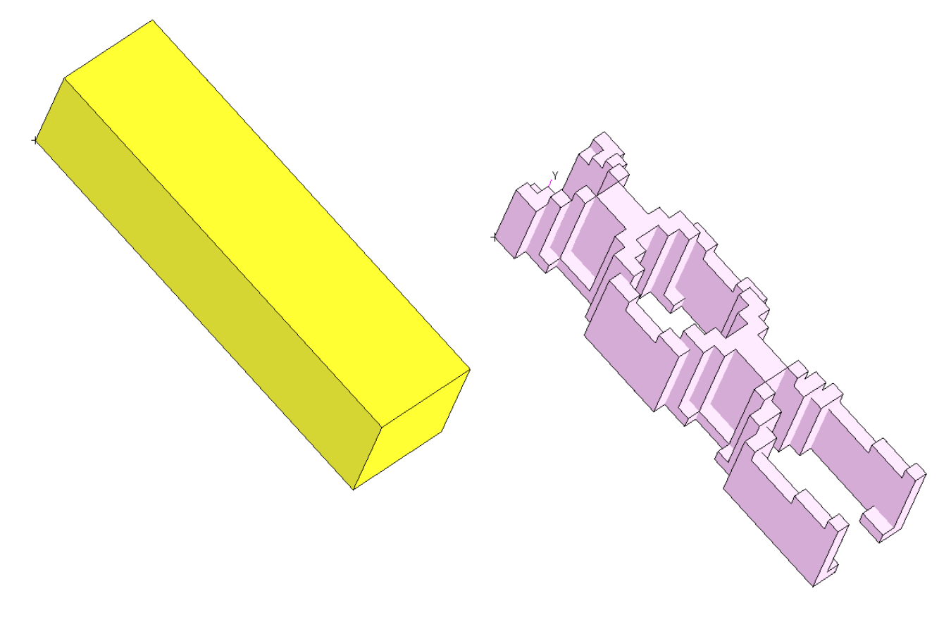
Example: Shape optimization of an aerospace mount. 
Shape optimization animation of an aerospace mount. 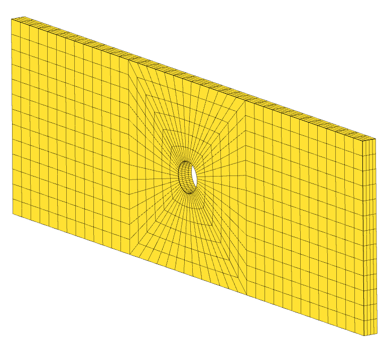
Example: Shape optimization of an open hole coupon.
|
||||||||||||||||||||
|
Validation
Before: Configuring a dynamic analysis is an extensive process. The MSC Nastran Dynamic Analysis User's Guide details an analysis strategy for defining a dynamic analysis. One step suggests applying a 1G gravity load in the x, y and z directions. Another step in the strategy involves performing a frequency response analysis at 0 Hz and comparing the results to an equivalent statics analysis. The process to do this traditionally involves manually editing the BDF files to remove damping, updating a FREQ entry to 0 Hz only, adding a statics subcase, and more. After: A new Model Validation web app has been introduced to help configure specific types of MSC Nastran validation runs, including the following.
Each option is available through a single checkbox. To request a 1G gravity load in the x, y and z directions, only one checkbox should be marked. To request a 0 Hz frequency response analysis and equivalent statics load case, only one checkbox should be marked. To remove damping from the model, only one checkbox should be marked. This new capability is featured in the tutorial titled Configure a 0 Hz Frequency Response and Statics Analysis. |
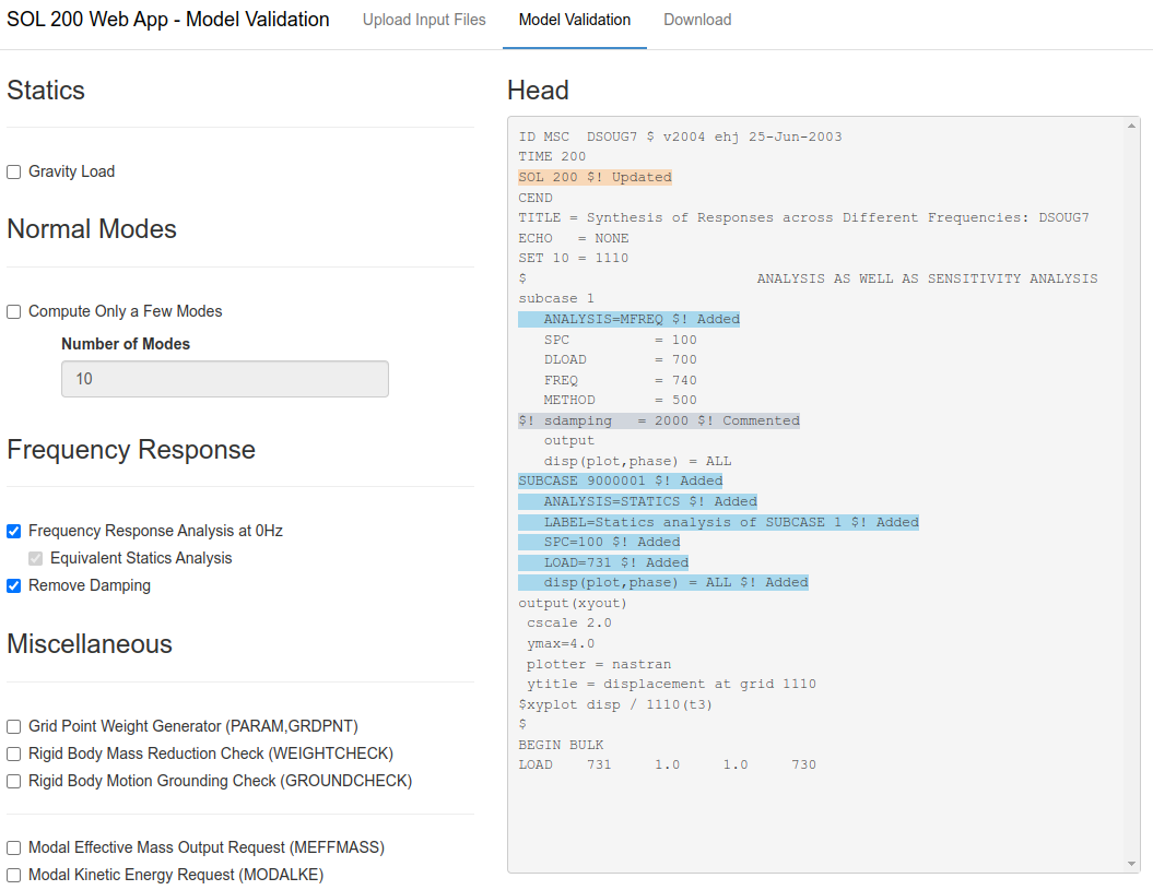
In the Model Validation web app, checkboxes are available to configure validation runs for statics, normal modes and frequency response analysis. |
V7.0.0
| New Capabilities and Descriptions | Image of New Capability |
|---|---|
|
Viewer – Ply Shape and Ply Number Optimization
Before: Composite material optimization is an elaborate and extensive process. One step in the procedure involves optimizing the ply shapes, or the location of ply drop-offs, to account for failure indices, buckling load factors, natural frequencies, and other design constraints. MSC Nastran allows defining composite plies via the PCOMP and PCOMPG entries. MSC Nastran’s topometry optimization capability allows for ply thickness optimization on an element-by-element basis. One significant difficulty in ply shape optimization is creating and managing hundreds of plies defined via dozens of PCOMPG entries across thousands of connector elements, e.g. CQUAD4, CTRIA3. After: This release introduces new capabilities to leverage topometry optimization results to decide the location of ply drop offs and produce optimal ply shapes. Tools are now available to spread ply shapes across critical regions of the composite, where a critical region is a region that significantly influences mechanical response such as failure indices, buckling load factors, natural frequencies, and other responses. The necessary PCOMPG entries and updates to the two-dimensional connector elements are automatically managed in the background. After optimal ply shapes are constructed, the number of plies for each ply shape must be determined. A new section named Ply Number Optimization Configuration is available and allows the configuration of ply number variables and assigning constraints on ply failure index, ply stress, ply strain and strength ratio. Options are available to constrain the total composite thickness or percentage of plies for a given angle, and produce a symmetric or balanced stack. After a ply number optimization, the PCOMPG entries are automatically updated with the newest number of plies. Additionally, a new option is available to visually display the thicknesses of plies. The capabilities mentioned are now available in the Viewer web app. These new capabilities are featured in the following tutorials, which are found in the Composite Laminate Optimization Tutorials section of the User’s Guide.
|
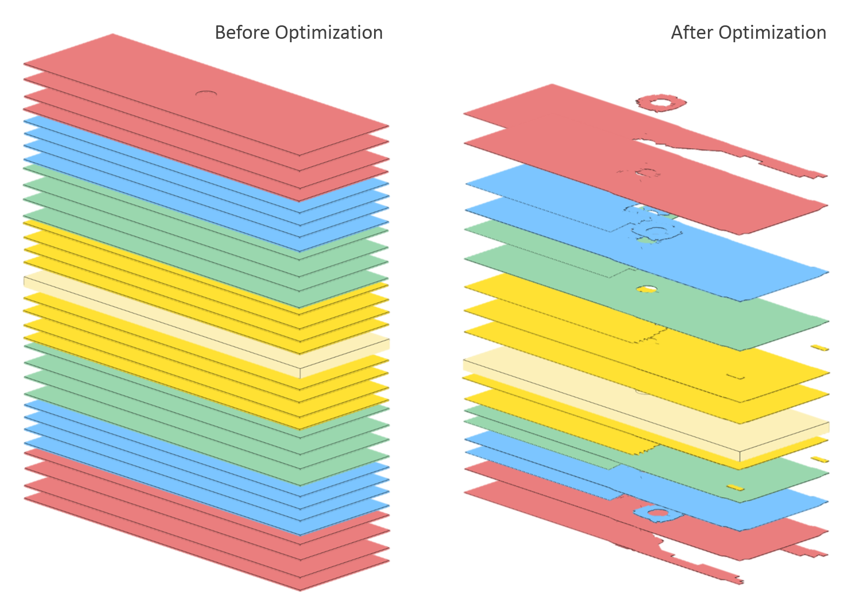
Left: Initial composite. Right: Final composite after ply shape and ply number optimization. |
|
Viewer – Topology Optimization
Before: Post-processing topology optimization results was done via the Topology Viewer web app. After: The Topology Viewer web app has been renamed to the Viewer web app. The Viewer web app is capable of post-processing topology optimization results. The Viewer web app is also capable of configuring optimal ply shapes and ply number optimizations. |
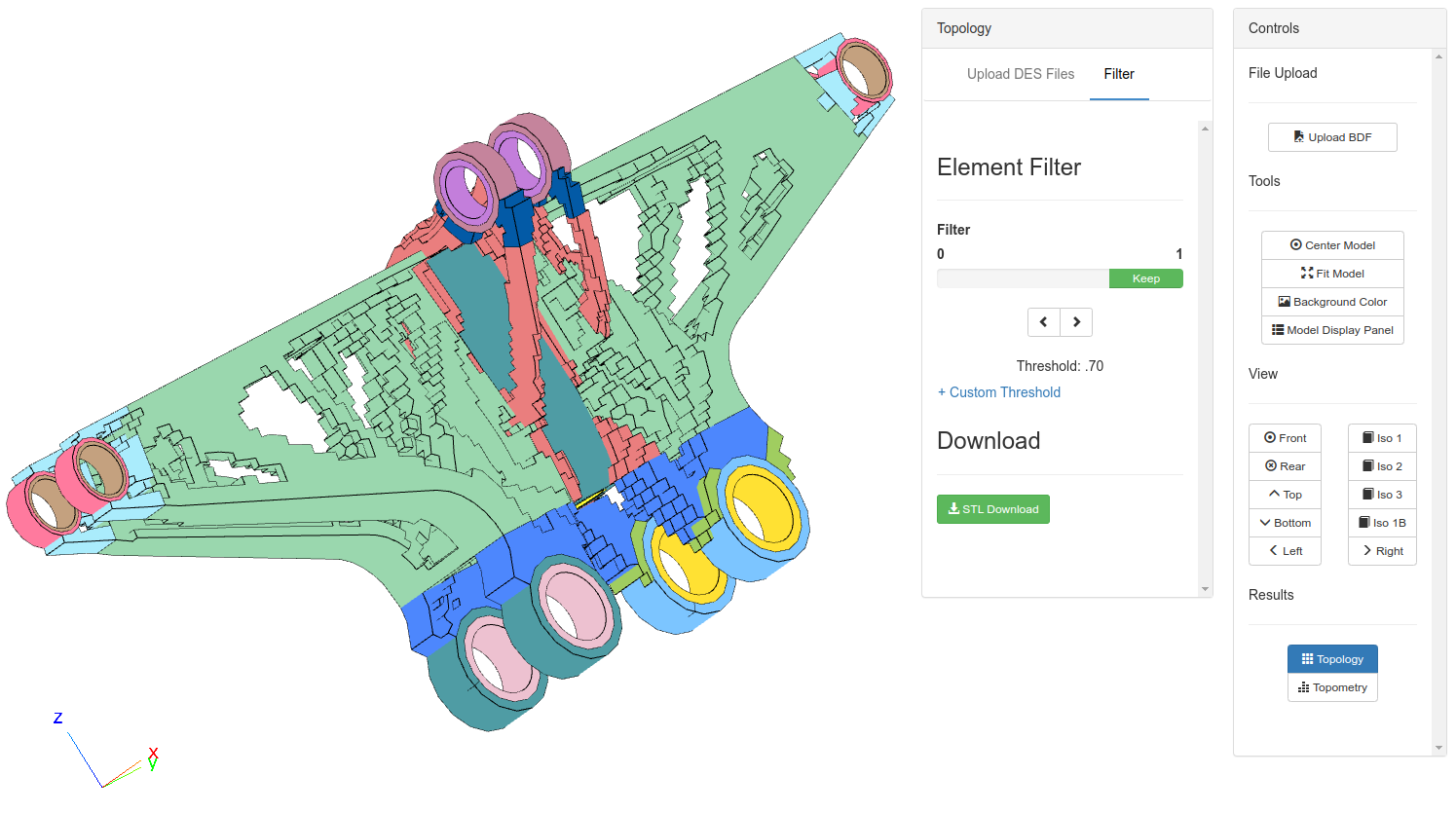
The Viewer web app is used to post-process topology optimization results 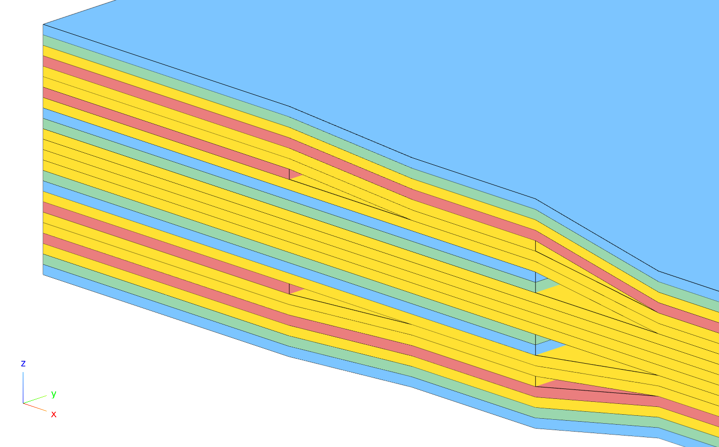
The Viewer web app is used to visually inspect the ply thicknesses |
|
Stacking Sequence Optimization
Before: Multiple manufacturing constraints exist for the stacking sequence of composite plies. For example, positive and negative angle plies, e.g. ±45°, are often paired together; certain angle plies should not be repeated more than four times; and the composite should be homogeneous as much as possible. After: A new Stacking Sequence web app has been added in this release. This web app allows for the stacking sequence optimization of composites defined either via the PCOMP or PCOMPG entries. Manufacturing constraints may be defined, the stacking sequence optimization may be executed, the resulting new composite may be visually inspected, and the PCOMP and PCOMPG entries are automatically updated. If the composite was defined via multiple PCOMPG entries, the stacking sequence of each relevant PCOMPG entry is automatically updated. This new capability is featured in the tutorial titled Composite Coupon – Phase E – Stacking Sequence Optimization. |
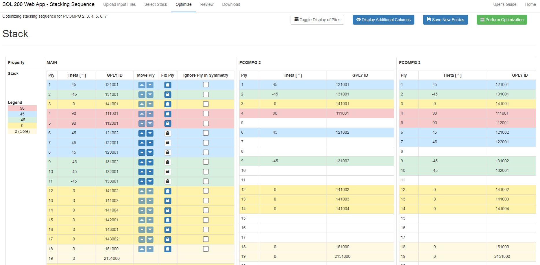
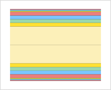
The Stacking Sequence web app is used to configure manufacturing constraints and perform a stacking sequence optimization. 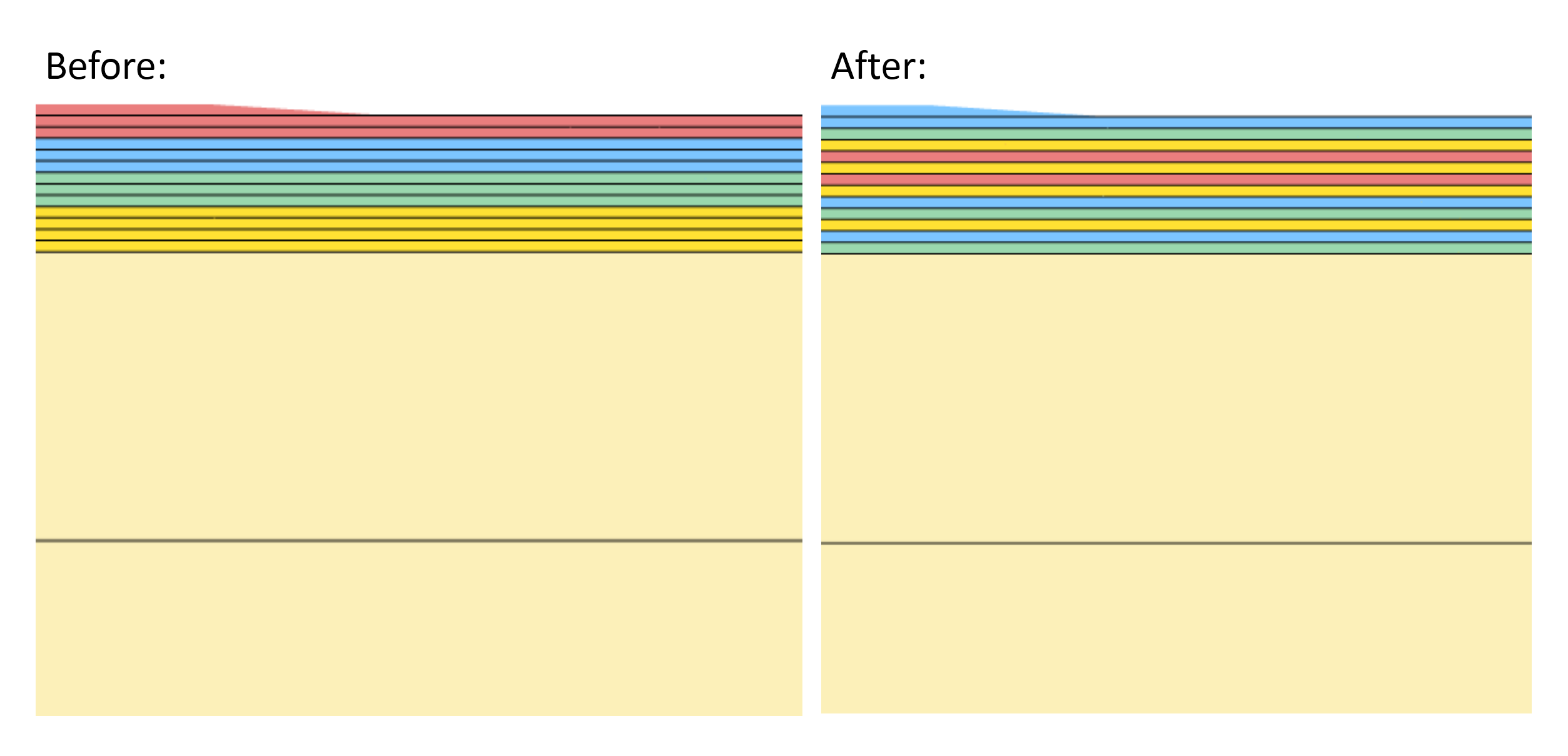
Left: The initial stacking sequence. After: The final stacking sequence after optimization. |
V6.5.0
| New Capabilities and Descriptions | Image of New Capability |
|---|---|
|
Remote Execution of MSC Nastran on Remote Systems
Before: Many organizations execute MSC Nastran on remote systems. For example, a user on Windows might move BDF files to a remote Linux system on the local network. Then the user manually starts MSC Nastran on the remote Linux system. The result files, including LOG, F06, OP2, etc., are manually copied to the local Windows system. The procedure requires the use of multiple programs, such as FTP and SSH programs. After: A new Remote Execution web app has been added in this release that achieves the same workflow of remotely running MSC Nastran, but does not require the use of FTP and SSH programs. With the Remote Execution web app, users may now upload input files, start MSC Nastran and download result files through a web browser. Also, a new Remote Execution Manager web app has been included and helps manage jobs on the remote system. This new capability is featured in the tutorial titled Remote execution of MSC Nastran on a remote operating system available on the local network. CommentsFor the Remote Execution web app to work properly, both the SOL 200 Web App and MSC Nastran must be installed on the same operating system. Both Linux and Windows operating systems are supported. The local and remote system may be either operating system. The Remote Execution web app operates by remotely executing the prod_version command, e.g. msc20224, msc20181, etc. The following example MSC Nastran jobs may be executed via the Remote Execution web app. If your MSC Nastran job is executed in a similar format, the job may be executed via the Remote Execution web app. msc20224 nastran name_of_input_file.bdf /msc/MSC_Nastran/2022.4/bin/msc20224 nastran name_of_input_file.bdf msc20181 MultiOpt name_of_input_file.xml /msc/MSC_Nastran/2018.1/bin/msc20181 MultiOpt name_of_input_file.xml Other execution jobs, such as Machine Learning and Parameter Study, are not executed via the prod_version command,
e.g. msc20224, and are not supported by the Remote Execution web app. The desktop executable, with shortcut name The following INCLUDE formats are supported by the Remote Execution web app. The paths must be relative. INCLUDE 'file_a.bdf' INCLUDE './file_a.bdf' INCLUDE './nested_directory/file_a.bdf' The following INCLUDE formats are NOT supported by the Remote Execution web app. INCLUDE 'C:\Users\usera\Downloads\nested_directory/file_a.bdf' INCLUDE '/nested_directory/file_a.bdf' INCLUDE '../nested_directory/file_a.bdf' INCLUDE TPLDIR:'nested_directory/file_a.bdf' INCLUDE formats that use backslashes (\) are NOT compatible on Linux. Pre-processors on Windows systems are known to create BDF files with INCLUDE entries that use backslashes. Exercise caution when uploading BDF files from a Windows system to a Linux system. An alternative is to use forward slashes (/) which are compatible on both Windows and Linux systems. The following USER FATAL MESSAGE is a sign of incompatibility. *** USER FATAL MESSAGE (fn: GETLIN) A requested INCLUDE file was not found. The Remote Execution web app allows you to download result files such as F06, LOG, etc. from the remote system. The nested directories on the remote system, which may contain the INCLUDE files, may not be downloaded in this web app version but will be addressed in a future release. One alternative to using INCLUDE files is to combine all the files together. This can be done by MSC Nastran with the following command. msc20224 nastran model.bdf expjid=yes The use of |
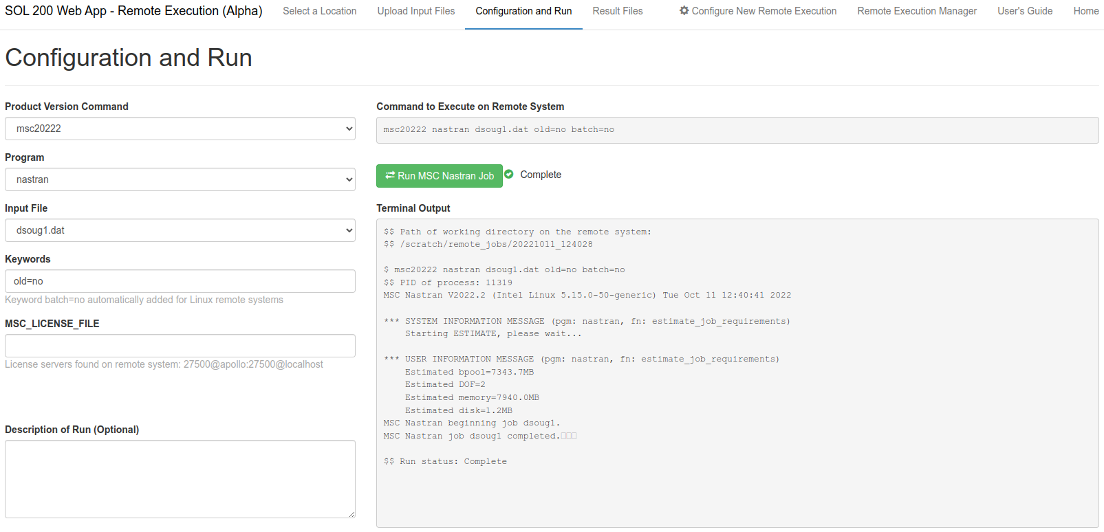
A web browser is used to upload BDF files to a remote system and run MSC Nastran. 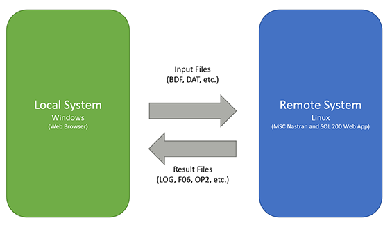
Diagram depicting the operations performed by the Remote Execution web app. |
|
Merging the Size and Topology Web Apps
Before: The Size and Topology web apps were separate. The Size web app allowed for the configuration of size, topometry and topography optimization. The Topology web app allowed for the configuration of topology optimization. Given this separation, it was difficult to configure a combined size, topometry, topography and topology optimization. After: The Size and Topology web apps has been merged together. The Size web app has been renamed to the Optimization web app. The Optimization features new secondary navigation bars to ease navigation of the variables, objective and constraints sections. This new capability is featured in a majority of SOL 200 tutorials available in the User's Guide. |
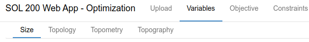
A new secondary navigation bar is displayed for the variables section. Sections available: Size, Topology, Topometry and Topography. 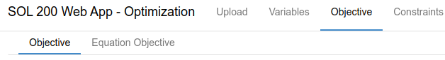
A new secondary navigation bar is displayed for the objective section. Sections available: Objective and Equation Objective. 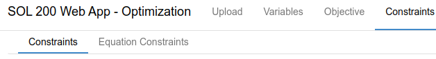
A new secondary navigation bar is displayed for the constraints section. Sections available: Constraints and Equation Constraints. |
V6.0.0
| New Capabilities and Descriptions | Image of New Capability |
|---|---|
|
PBMSECT Web App
Before: Arbitrary beam cross sections (ABCS) may be defined via the PBMSECT or PBRSECT entries, but requires: carefully configuring the entry's keywords OUTP, BRP, T, INP, CORE, LAYER and NSM; and the creation of SET1, SET3 and POINT bulk data entries. The ABCS is displayed by running MSC Nastran and generating the PostScript (PS) and AAA_xxyyy_zz.bdf files. This is a multi-step and iterative process. After: A new PBMSECT web app has been developed and is used to visually construct arbitrary beam cross sections. Internally, the PBMSECT web app will create and manage the PBMSECT, PBRSECT, POINT and SET1 entries. Existing BDF files maybe uploaded to the PBMSECT web app and new or existing cross sections may be created and edited. This new capability is featured in the tutorials titled Introduction to the PBMSECT Web App, Examples of arbitrary beam cross sections with PBMSECT and PBRSECT, Composite Arbitrary Beam Cross Section, Arbitrary Beam Cross Section Optimization. |
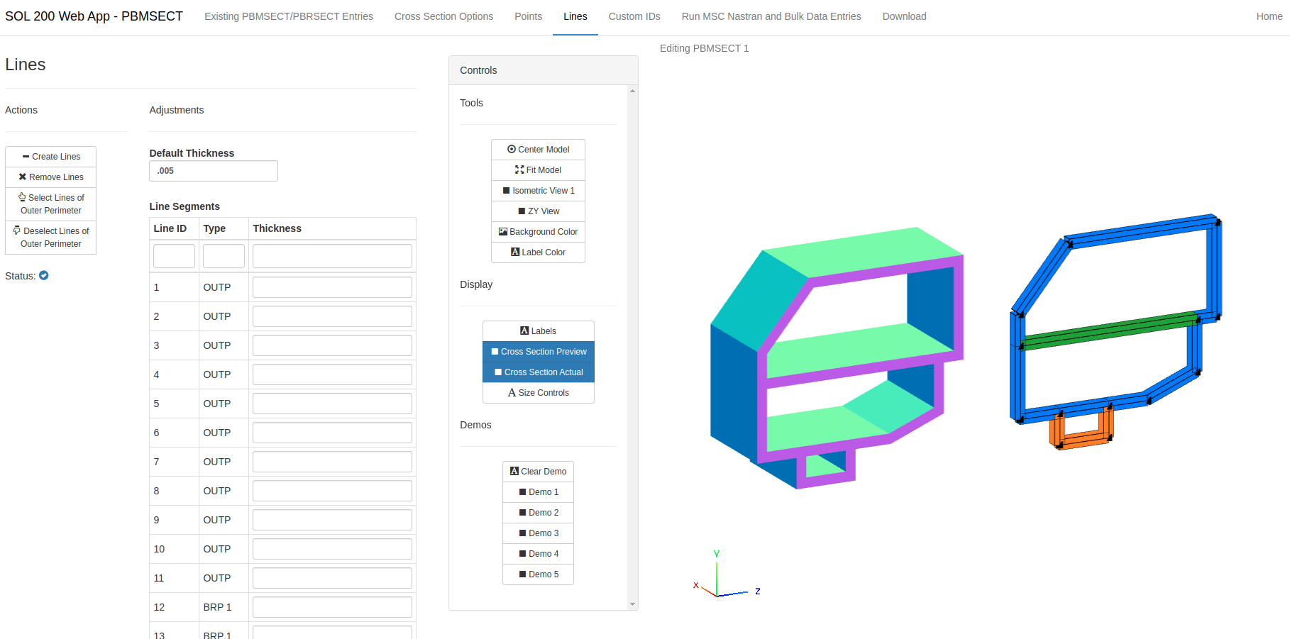
A GUI is used to define the points and line segments of an arbitrary beam cross section. A preview and an actual MSC Nastran generated cross section are displayed. |
|
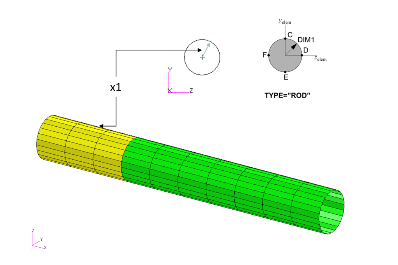
Beams Viewer
Before: Utilizing MSC Nastran's 1D elements requires carefully configuring values such as offset or orientation vector and is often done with no visual confirmation. After: A new web app named the Beams Viewer is available to display 1D and 2D elements, including: CONROD, CROD, CBAR, CBEAM, CBEAM3, CBEND, CTUBE, CTRIAi and CQUADi elements. The Beams Viewer may also be used to display internal element forces such as shear forces or moments. It should be noted that the Beams Viewer has no capability to edit 1D elements. The Beams Viewer is ideally used to visually confirm 1D elements. Due to web browser limitations, a maximum BDF file size of 200KB may be uploaded to the Beams Viewer. This new capability is featured in the tutorial titled Arbitrary Beam Cross Section Optimization. |
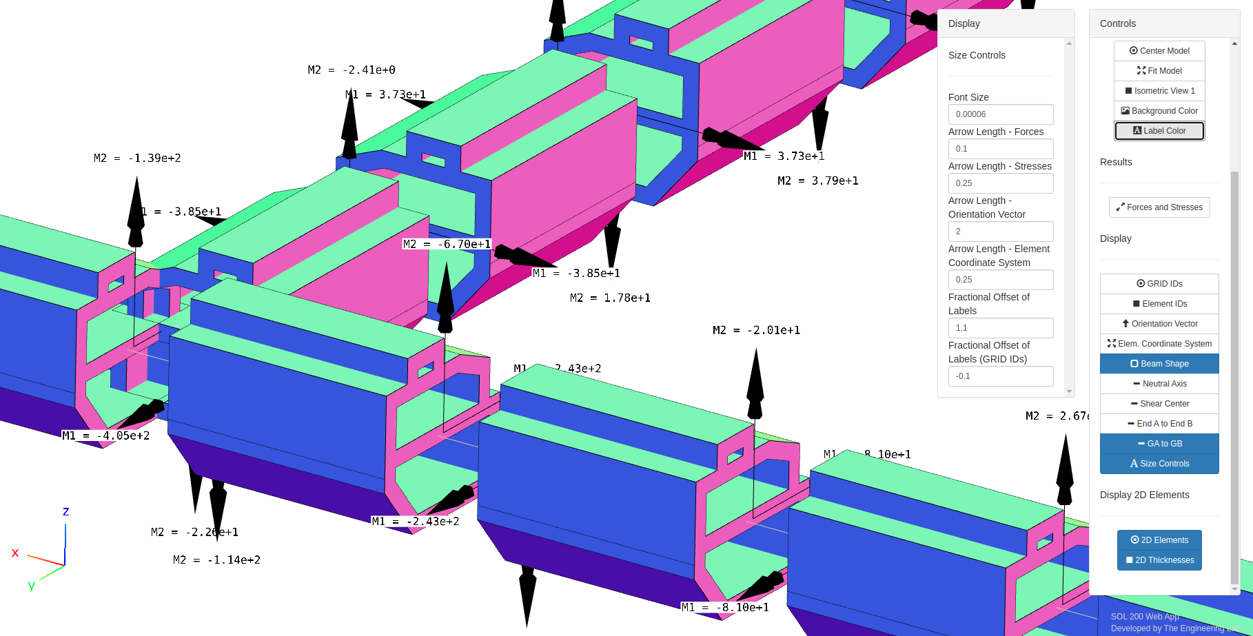
A arbitrary beam cross section is displayed, along with internal element forces and moments. |
|
Batch Execution of MSC Nastran With Varying Integer Fields
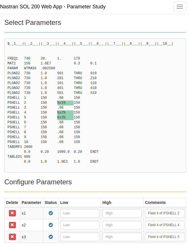
Before: The Machine Learning web app is capable of configuring multiple batch runs for MSC Nastran. Previously, any field that contains a real value, i.e. contains a decimal character, may be configured as a parameter. If a field contains an integer value, i.e. contains only digits and no decimal, such fields could not be configured as parameters. After: Integer fields may now be set as parameters. Users may configure multiple batch runs for MSC Nastran while varying the integer value of selected fields. One example of this new capability involves configuring multiple batch runs to vary the locations of concentrated masses. The goal is to determine the optimal location of concentrated masses. This new capability is featured in the tutorials titled Parameter Study, Varying the Location of Concentrated Masses and Parameter Study, Varying the Position of Extra Supports. |
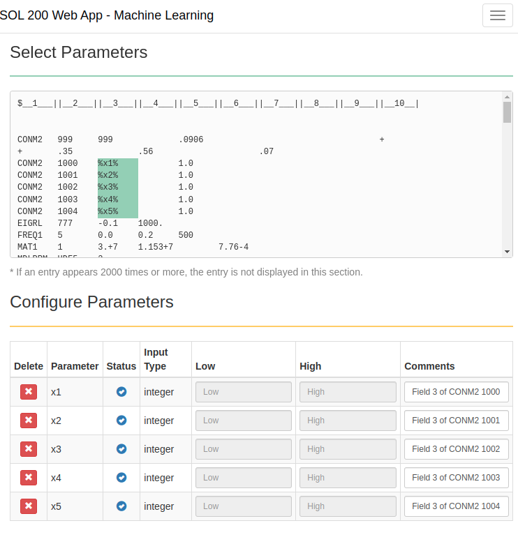
In this example, the GRID positions of concentrated masses (CONM2) are varied for multiple batch runs of MSC Nastran. |
|
Dynamic Stiffness Auto Plots After Optimization
Before: Version 5.6.0 of the SOL 200 Web App made available the new DRESP1 response type dynamic stiffness (DYSTIFF). The HDF5 Explorer automatically generates certain XYPLOTs but dynamic stiffness plots were not automatically generated. After: After an optimization is performed, the HDF5 Explorer will now automatically create the XYPLOTs for dynamic stiffness. Auto plot generation for dynamic stiffness responses works best for MSC Nastran 2022.1 or newer. |
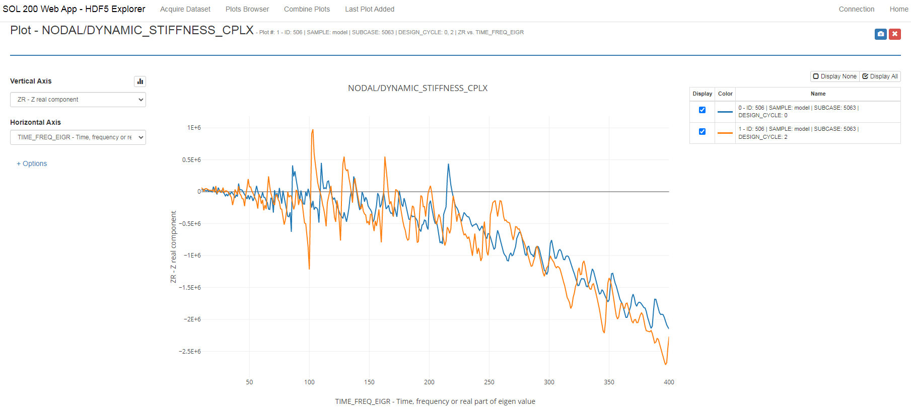
An XYPLOT of the dynamic stiffness response, before and after optimization, is automatically generated via the HDF5 Explorer. |
V5.6.0
| New Capabilities and Descriptions | Image of New Capability |
|---|---|
|
Support for dynamic stiffness as a response (DRESP1 RYTPE=DYSTIFF)
Before: Optimizing a model for dynamic stiffness previously required the creation of DRESP2, DRESP1 and DEQATN entries to create the dynamic stiffness response. MSC Nastran 2021.4 introduced a new type-1 response type (DRESP1 RTYPE=DYSTIFF) corresponding to the dynamic stiffness. The new dynamic stiffness response type reduces the need to create multiple DRESP2, DRESP1 and DEQATN entries. After: The new response type for dynamic stiffness (DRESP1 RTYPE=DYSTIFF) may now be created in this web app. Users can configure optimizations to maximize or constrain dynamic stiffness responses. This new capability is available in the Size web app and is found when creating DRESP1 entries. The DRESP1 RTYPE=DYSTIFF option is only available in MSC Nastran 2021.4 or newer. |
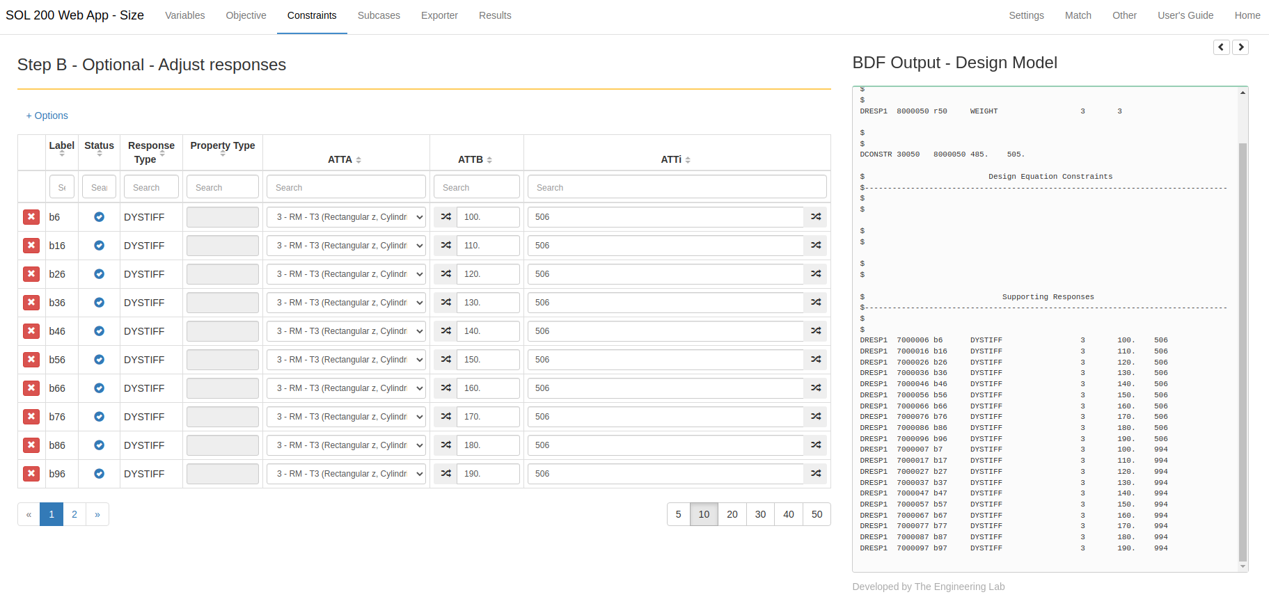
Multiple DRESP1 entries corresponding to the dynamic stiffness (RTYPE=DYSTIFF) are created. |
|
Support for DTABLE
Before: DEQATN entries may be generated in the Size and Topology web apps. If a user had a need to use constants in the DEQATN entry, the constants were manually typed into the EQAUTION field. Any adjustments to the constants required the editing of the EQUATION field on the DEQATN entry. After: The DTABLE entry is now supported. Users may now create constants via the DTABLE entry and use these constants in DEQATN, DVxREL2 and DRESP2. Any edits to the constants is done to the DTABLE entries instead of the DEQATN entries. This new capability is available in the "Other" section of the Size and Topology web apps. |
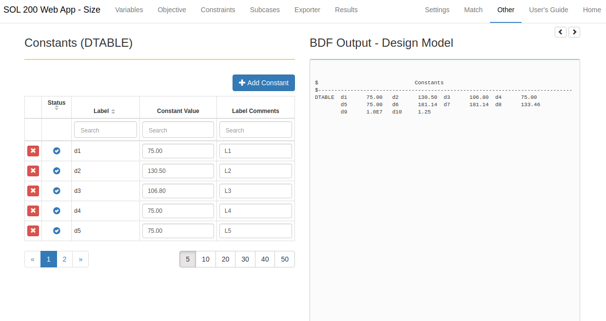
The web app is used to configure the DTABLE entry which specifies constants that may be used in the DRESP2, DEQATN, DVPREL2, DVCREL2 and DVMREL2 entries. |
|
Persistence of Unsupported Fields
Before: The Size and Topology web apps support a majority of the fields across bulk data entries for SOL 200, e.g. DESVAR, DRESP1, etc. Certain fields, such as the DELXV field on the DESVAR entry, are not supported by the web app since the default values (blank) are sufficient for a majority of cases. On BDF file import, the Size and Topology web apps remove these fields. For example, if a BDF file had a DESVAR entry with the DELXV field, upon import, the Size web app would strip away the DELXV field. After: To preserve as much as possible information from the original BDF, the following fields may now be uploaded to the web app and are untouched. After download, the same untouched fields are present in the BDF files.
|
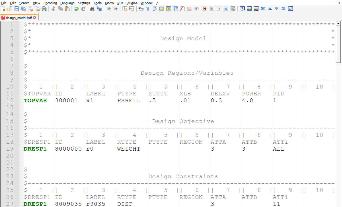
After the design_model.bdf file is downloaded, the extra fields, e.g. XINIT, XLB, DELXV and POWER, on the TOPVAR entry are preserved. |
|
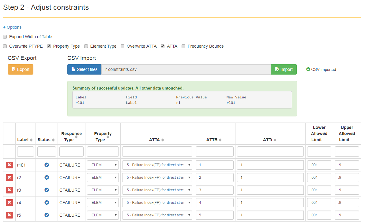
Improvement to CSV Import
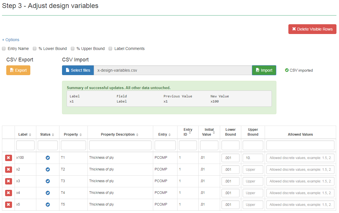
Before: The Size and Topology web apps includes a CSV Export/Import interface. The CSV Export/Import interface allows one to use a CSV file to edit variables and design constraints (DESVAR, DVXREL1, DVXREL2, DRESP1, DRESP2, DCONSTR). In prior versions of the web app, the CSV Import capability was difficult to use. Specifically, in some scenarios, the CSV file was limited to one import. After the first import, the CSV file was no longer imported. After: The CSV file may now be imported continuously. Users will find it easier to use a CSV file to edit or create variables and constraints. This new capability is featured in the tutorials titled CSV Export and Import for Design Variables, Responses and Constraints and Model Matching, Frequency Response Analysis. |
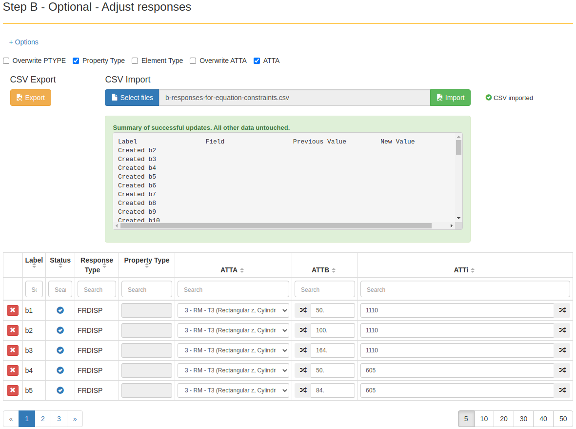
A CSV file is imported and used to create multiple DRESP1 entries. |
|
Improvement to Free Field Format Support
Before: The free field format uses both commas and spaces to separate data fields. In prior versions of the web app, the free field format was supported, but only supported commas as separators. After: This version now supports spaces as separators in free field formatted bulk data entries. |
pbeaml, 100, 200,, I
      , 50., 45., 45., 5., 5. 5.
$                          ^^^^
$ In the PBEAML entry above, fields 16 and 17
$ are separated by a space instead of a comma.
|
V5.5.0
| New Capabilities and Descriptions | Image of New Capability |
|---|---|
|
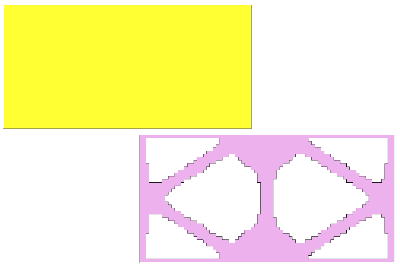
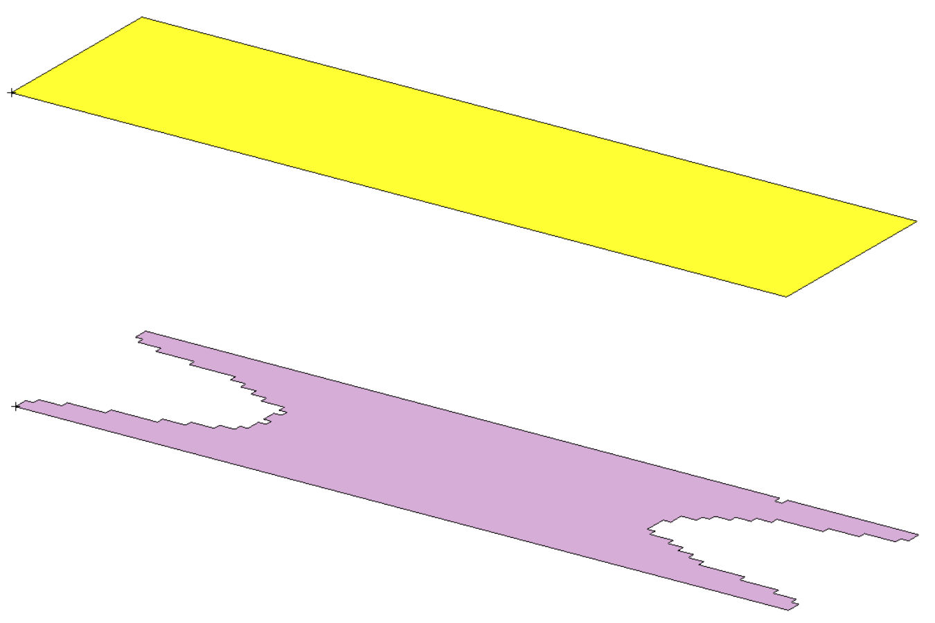
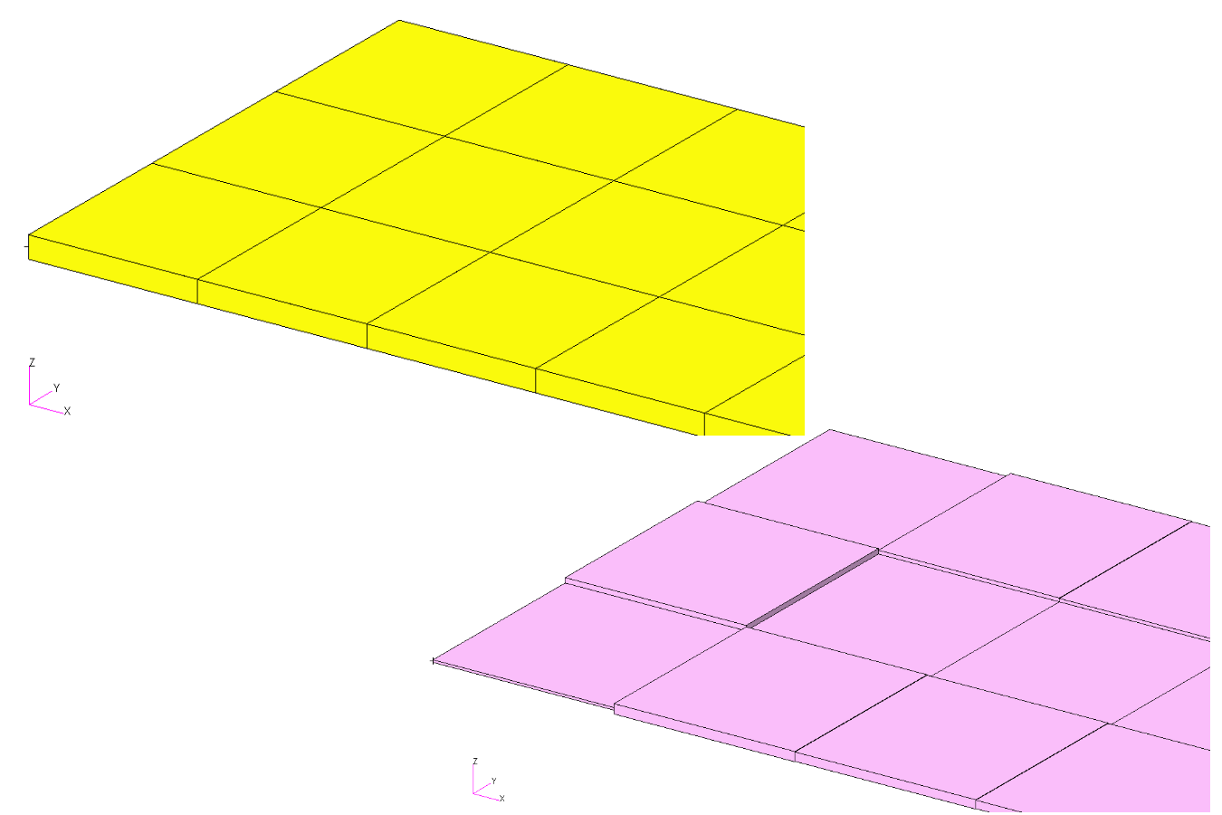
Support for Topography/Bead Optimization
Before: MSC Nastran has an existing capability to perform Topography/Bead optimization. In prior versions, Topography optimization was not supported by the SOL 200 Web App. After: Topography optimization is now supported. The SOL 200 Web App now supports the existing topography optimization bulk data entry BEADVAR. This new capability is featured in the tutorial titled MSC Nastran Topography Optimization - Bead or Stamp Optimization. |
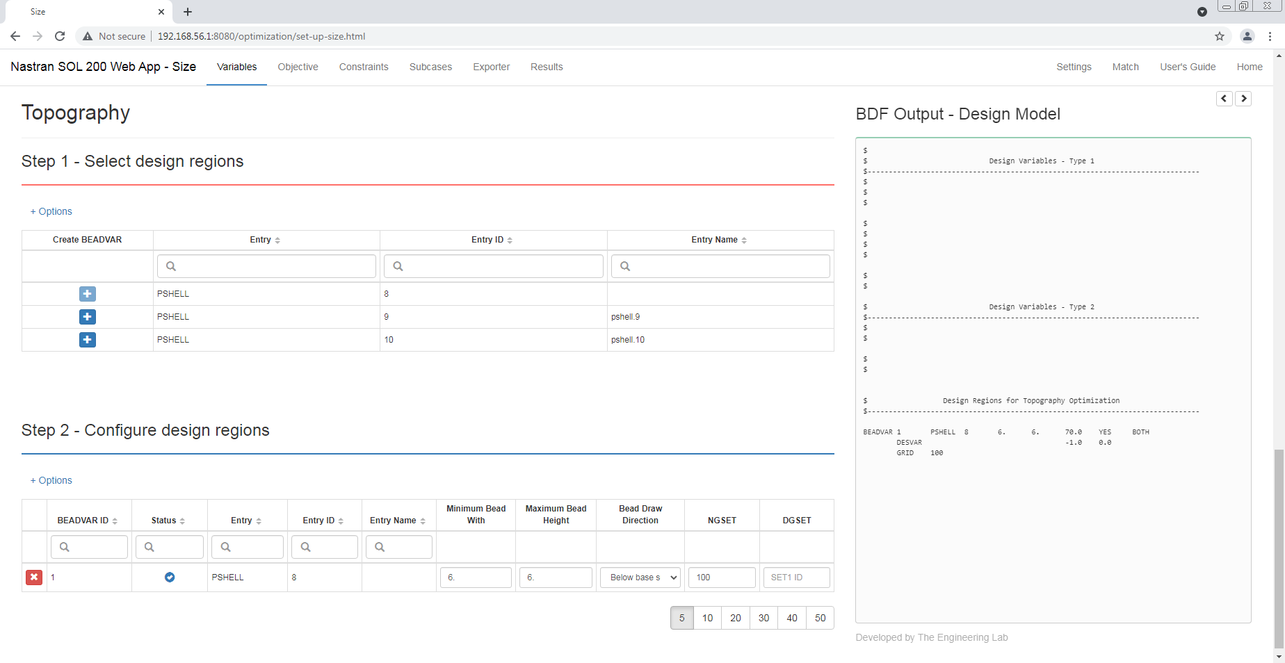
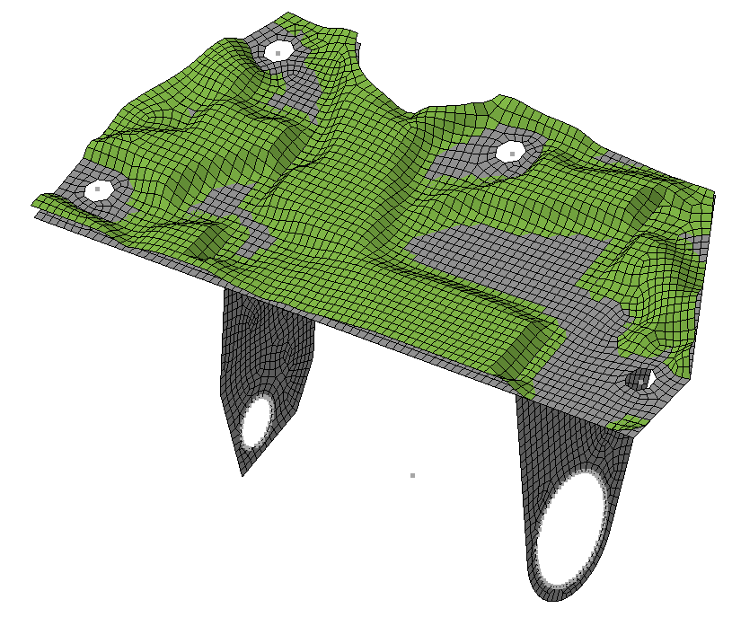
The web app is used to configure the BEADVAR entry which specifies the topography design region. 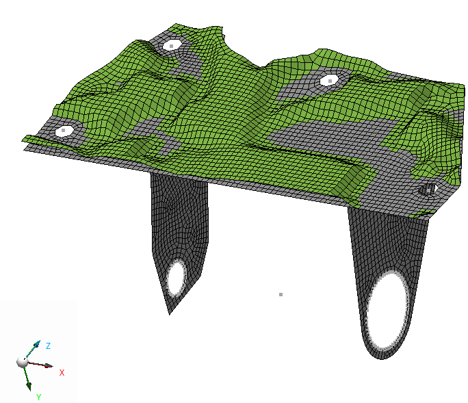
The initial (grey) and final/optimized (green) designs are superimposed. |
|
Support for Extracting Responses from H5 Files Generated at Remote Locations, e.g. server or other desktops
Before: The Machine Learning web app enables the configuration of batch MSC Nastran runs and the collection of responses by extracting responses from the H5 file. For example, the Machine Learning web app may be used to configure dozens or hundreds of MSC Nastran runs. Upon download, the necessary BDF files and a specialized, portable desktop app are downloaded in a file typically named nastran_working_directory.zip. For each run, the desktop app will automatically execute MSC Nastran and collect the responses in a CSV file. The capability of extracting responses from the H5 file required that MSC Nastran be executed locally. If MSC Nastran was executed in a remote location and outside the desktop app, say a server, the desktop app cannot be used to extract the responses from the H5 files. After: The desktop app has been updated to support the reading of H5 files generated outside the desktop app. The new workflow is as follows:
|
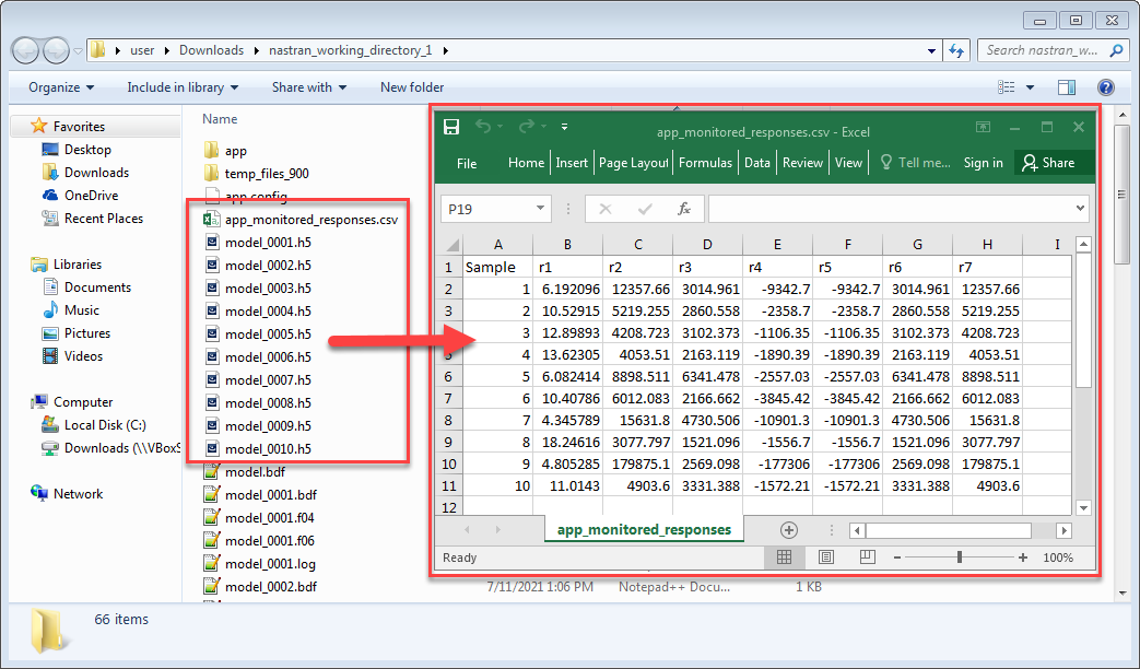
The desktop app extracts the responses from the H5 files and saves the responses to a CSV file. |
|
Support for Design Models Created Outside the Web App
Before: Prior to v3.5.0 of the SOL 200 Web App, web app for short, Bulk Data Files (BDF) generated by other pre-processors were not compatible with the web app. The v3.5.0 release of the web app introduced the Converter web app, which was used to convert SOL 200 BDFs generated by separate pre-processors. The workflow was as follows.
After: The Converter web app has been merged into the Size, Topometry and Topology web apps. Now, BDFs created by separate pre-processors may be directly uploaded to the Size, Topometry and Topology web apps. There is no need to use the separate Converter web app when handling BDFs created by separate tools. The new workflow is as follows.
This new capability may be explored as follows. The MSC Nastran Test Problem Library contains existing SOL 200 examples dsoug1.dat, dsoug2.dat and dsoug4.dat. These SOL 200 examples may now be directly uploaded to the Size, Topometry and Topology web apps. In prior versions of the web app, these examples were seen as incompatible by the web app and required the use of the separate Converter web app. Reminder! The web app only reads and converts bulk data entries listed in the section titled Supported MSC Nastran Entries. All other entries are ignored, e.g. DRESP3, DVBSHAP, etc. |
$ Incompatible Entry DRESP1 20 W WEIGHT $ Compatible Entry (After Conversion) DRESP1 8000000 r0 WEIGHT |
V5.0.0
| New Capabilities and Descriptions | Image of New Capability |
|---|---|
|
Machine Learning for Nonlinear Response Optimization
Before: Gradient-based optimization has been demonstrated to be a reliable method in linear response optimization. For example, MSC Nastran SOL 200's optimization capability is applicable to solution sequences, 101, 103, 105, 107, 108, 110, 111, 112, 144 and 145. If a practitioner is interested in nonlinear response optimization, say with responses from SOL 400, gradient-based optimization is not as reliable. After: Bayesian optimization is an alternative to gradient-based optimization. Bayesian optimization is an optimization strategy that bases its design selection on "what we know so far." The strategy involves constructing a surrogate model, via Gaussian process regression, and constructing acquisition functions, which quantifies where in the design space a better design point may exist. Bayesian optimization is commonly used in scenarios where response acquisition is expensive, like it is in finite element analysis. Bayesian optimization is an excellent option for nonlinear response optimization.
This new capability is featured in any tutorial with the phrase Machine Learning in the title. Refer to the Machine Learning Tutorials in the User's Guide. |
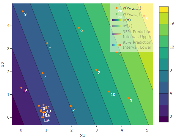
Runs 1-10 are used to train the initial surrogate model. Runs 11-20 are the active learning iterations. 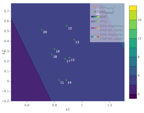
A close look at runs 11-20 reveals the candidate points are clustered together. This is indication that the optimum is being approached. |
|
Prediction Analysis via Gaussian Process Regression
Before: In some instances, finite element analysis can require hours to complete. If there is a need to run multiple finite element (FE) analyses, days or weeks may be required. Methods to determine the FE solver output with a limited number of FE analyses are desired. After: Now available is the surrogate modeling technique Gaussian process (GP) regression. The surrogate model is used to predict the output of the FE solver. These predictions are computed in seconds and is a contrast to FE analyses that sometimes span hours. To construct a GP based surrogate model, the FE solver is used to evaluate an FE model at various FE model configurations. The resulting outputs are used to construct the surrogate model. This capability is now available in the Prediction Analysis web app. For example, if it is desired to vary two parameters of the FE model and 5 runs per parameter are considered, a total of 10 solver runs are performed. All 10 runs produce output responses. The 10 different FE configurations, termed inputs, and output responses are used to train the surrogate model via Gaussian process regression. The surrogate model is then used to predict the response at different parameter configurations. It should be noted that the Machine Learning web app can be used to configure multiple MSC Nastran runs and collect the output responses. The different FE configurations, or inputs, and output responses serve as the training data that the Prediction Analysis web app uses to construct the surrogate models. This new capability is featured in any tutorial with the phrase Prediction Analysis in the title. Refer to the Machine Learning Tutorials in the User's Guide. |
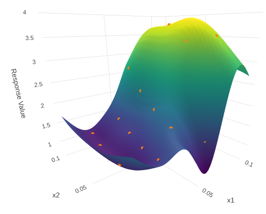
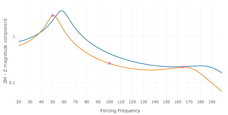
Response surface of the surrogate model. The model represents a frequency response. Twenty MSC Nastran runs were executed to generate the training data and are indicated by the orange points. 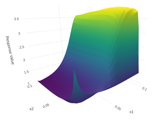
Response surface of the true function. Note the similarity between the true and prediction function (surrogate model). Over 1,000 MSC Nastran runs were executed to generate this response surface of the true function. |
V4.0.0
| New Capabilities and Descriptions | Image of New Capability |
|---|---|
|
Parameter Study Web App
Before: Improving a mechanical design is an extensive process and employs multiple techniques, such as sensitivity analysis, optimization, and parameter study. MSC Nastran has SOL 200, capable of optimization, but is limited to linear solution sequences in the 100 series, for example, SOL 101 and 103. This optimization capability does not support solution sequences such as SOL 109 and SOL 400, the advanced nonlinear analysis solution sequence. An alternative is to perform a parameter study. The process involves generating numerous configurations of a finite element model, then using MSC Nastran to evaluate each configuration. For example, a user decides to analyze a finite element model ten times, each with a different material or property, such as thickness. Creating multiple design configurations, collecting results, and reviewing results is a tedious, time-consuming manual process. After: This release features a new web application named Parameter Study and enables users to configure multiple design configurations, run MSC Nastran for each configuration, and track FEA output automatically. This new web app is compatible with any solution sequence, including SOL 400, and significantly improves the efficiency and productivity of a parameter study. The workflow is as follows:
This new capability is featured in any tutorial listed in the section named Machine Learning Tutorials. |
|
|
HDF5 Explorer
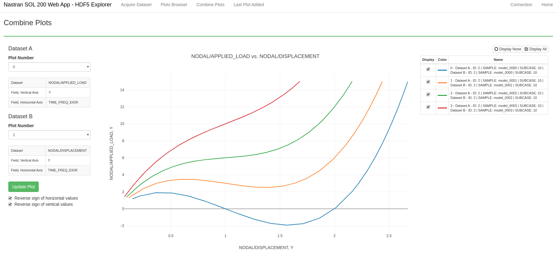
The HDF5 Explorer features new enhancements. Ease of UseBefore: The process of starting the HDF5 Explorer required multiple steps. A desktop application was first downloaded and executed. When executed, the desktop app began streaming data from the H5 file to the web browser. After: H5 files can be directly uploaded to the web browser. The need to download the desktop application is not necessary but remains as an alternative option. This new capability is featured in the tutorial titled Use the HDF5 Explorer to Create Plots. CapacityBefore: Only one H5 file could be accessed by the HDF5 Explorer. After: Multiple H5 files can be uploaded and accessed by the HDF5 Explorer. Users can now compare results between different H5 files. FunctionalityBefore: There is a desire to create Load vs. Displacement plots, but the HDF5 Explorer did not support this type of plot in prior versions. After: A new capability has been introduced that enables users to combine multiple plots. The HDF5 Explorer can now create a Load vs. Displacement plot by combining a Load plot with a separate Displacement plot. This new capability is featured in the tutorial titled Parameter Study, Nonlinear Buckling. |
|
V3.5.0
| New Capabilities and Descriptions | Image of New Capability |
|---|---|
|
Topology Viewer
Before: After a topology optimization, the topology results could only be displayed and reviewed by a separate, traditional post processor. After: A web driven Topology Viewer has been created. The viewer allows users to review topology results and export the results to the STL file format. |
|
|
HDF5 Explorer
Before: In a previous release, the Dynamic Plots App was used to extract results from the MSC Nastran HDF5 (.h5) file and generate plots. The Dynamic Plots App was limited to only frequency response analysis plots. After: The Dynamic Plots App has been expanded beyond frequency response analysis results and allows users to interactively browse the HDF5 result file. In addition, data from the HDF5 file can be extracted to a CSV file or plots may be generated. |
|
|
PCH to BDF - PCOMP Topometry Results Support
Before: During a Size or Topometry optimization, a new PCH file is created with updated Bulk Data Entries. The PCH to BDF web app allows users to automatically transfer new entries from the PCH file to the BDF files. This capability was limited to properties used during a Size optimization. If a user performed a Topometry Optimization on PCOMP entries for composite optimization, the PCH to BDF web app could not be used to transfer entries from the PCH file to the BDF files. After: The PCH to BDF web app now supports Topometry optimization results for PCOMP entries. During the automatic transfer process, two steps are performed: 1) The new PCOMP entries are transferred to the BDF files 2) The respective 2D elements, e.g. CQUAD4, are updated to point to the new PCOMP IDs. |
Before: CQUAD4 1 1 [...] PCOMP 1 [...] After: CQUAD4 1 10000001 [...] PCOMP 10000001 [...] |
|
Free Field Format Support
Before: Properties, such as thickness, area, Young's modulus, etc., can be set as design variables. The web app extracts these properties from bulk data entries as long as the entry is in the small or large field format. Any property within an entry in the free field format was ignored. After: Properties can now be extracted from entries in the free field format. |
$ Entry formatted in the Free Field Format PCOMP,2,,,13000.,HILL,,, ,1,.01,85.,YES,1,.01,-85.,YES ,1,.01,60.,YES,1,.01,-60.,YES ,1,.01,60.,YES,1,.01,-60.,YES ,1,.01,85.,YES,1,.01,-85.,YES |
|
Converter App
Before: The web app uses specific sets of identification numbers(IDs) for many bulk data entries. These entries include, but are not limited to: DESVAR, DRESP1, DRESP2, etc. Design models created by separate tools or manually edited are not compatible with the web app and cannot be uploaded to the Size or Multi Model Optimization web apps. After: A new Converter App has been created that converts incompatible design models to compatible versions. Converted design models can then be uploaded to the Size or Multi Model Optimization web apps. |
$ Incompatible Entry DRESP1 20 W WEIGHT $ Compatible Entry (After Conversion) DRESP1 8000000 r0 WEIGHT |
|
REPCASE Support
Before: If a REPCASE command exists in the Case Control Section, an ANALYSIS command must be specified. In previous web app versions, the ANALYSIS command was only added to SUBCASE sections, but not REPCASE sections. After: The ANALYSIS command is automatically inserted if REPCASE is detected. |
$ Example of a SUBCASE with a REPCASE command SUBCASE 3 ANALYSIS = STATICS DESSUB = 40000003 $ DRSPAN Slot SUBTITLE=Static Analysis 1 LABEL = LOAD CONDITION 1 LOAD = 300 REPCASE 4 ANALYSIS = STATICS LABEL= Static Analysis 1 Repcase DISPLACEMENT(PLOT) = ALL |
V3.0.0
| New Capabilities and Descriptions | Image of New Capability |
|---|---|
|
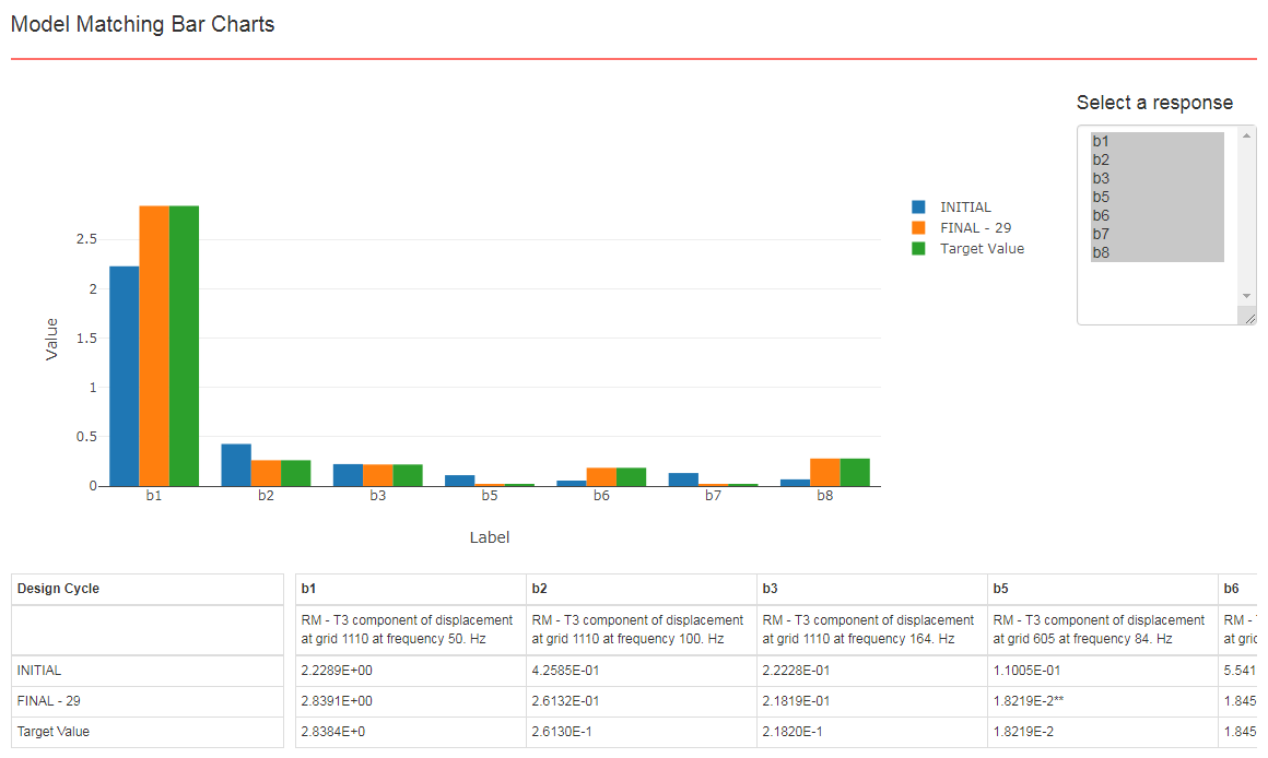
Model Matching
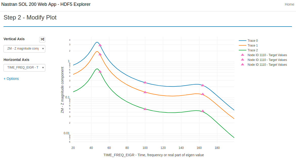
Before: To configure a design model for model matching, an Equation Objective or Equation Constraint must be explicitly defined. The process is laborious once multiple responses are configured for model matching. After: A new model matching table has been introduced and streamlines the design model creation process. With the new table, and for each individual response, users need to configure 3 items for model matching: target value, inclusion in the objective and max allowed error. Internally, the web app automatically generates and manages the necessary Equation Objective and/or Equation Constraints. The Auto Execute program has also been updated to support model matching. Once an optimization for model matching is complete, the Auto Execute program will automatically upload model matching results to the web app and display comparisons between the INITIAL, FINAL FEA values and the target values. This new capability is featured in the tutorials titled Using MSC Nastran Optimization for Model Matching / System Identification and Model Matching, Frequency Response Analysis. |
|
|
CSV Export/Import for Other Responses, Constraints and Equation Constraints (Official Release)
Before: The CSV capability for Other Responses, Constraints and Equation constraints was previously in an experimental state. After: This CSV Capability is now officially complete and available. This new capability is featured in the tutorial titled CSV Export and Import for Design Variables, Responses and Constraints. |
|
V2.5.0
| New Capabilities and Descriptions | Image of New Capability |
|---|---|
|
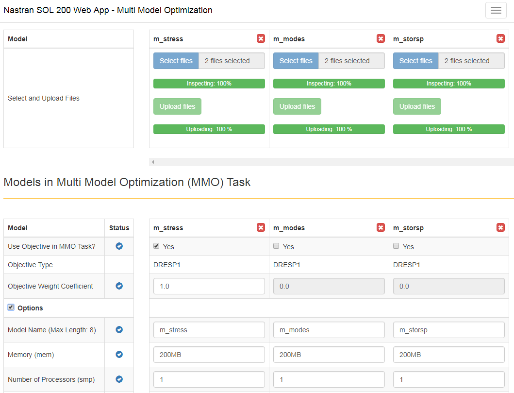
Multi Model Optimization
Before: Multi Model Optimization (MMO) could not be configured in the SOL 200 Web App. After: A new MMO Web App has been introduced and allows the configuration and execution of MMO. The new MMO Web App is accessible from the homepage. This new capability is featured in the tutorial titled Multi Model Optimization. |
|
|
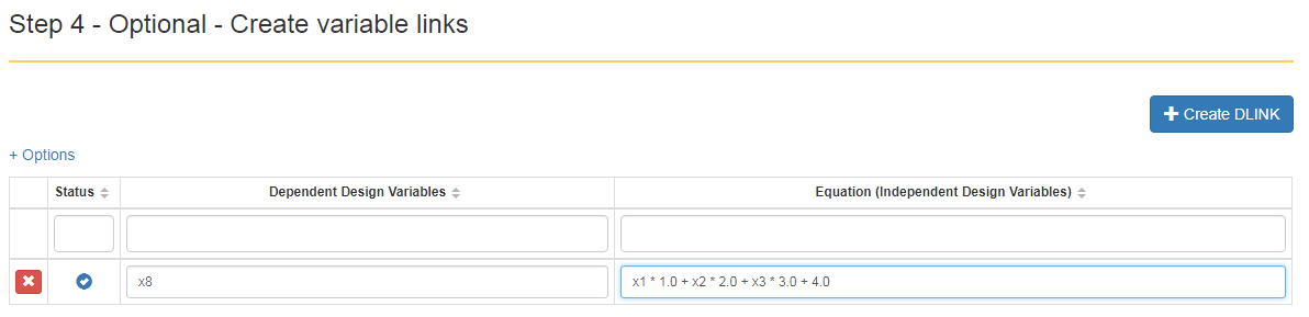
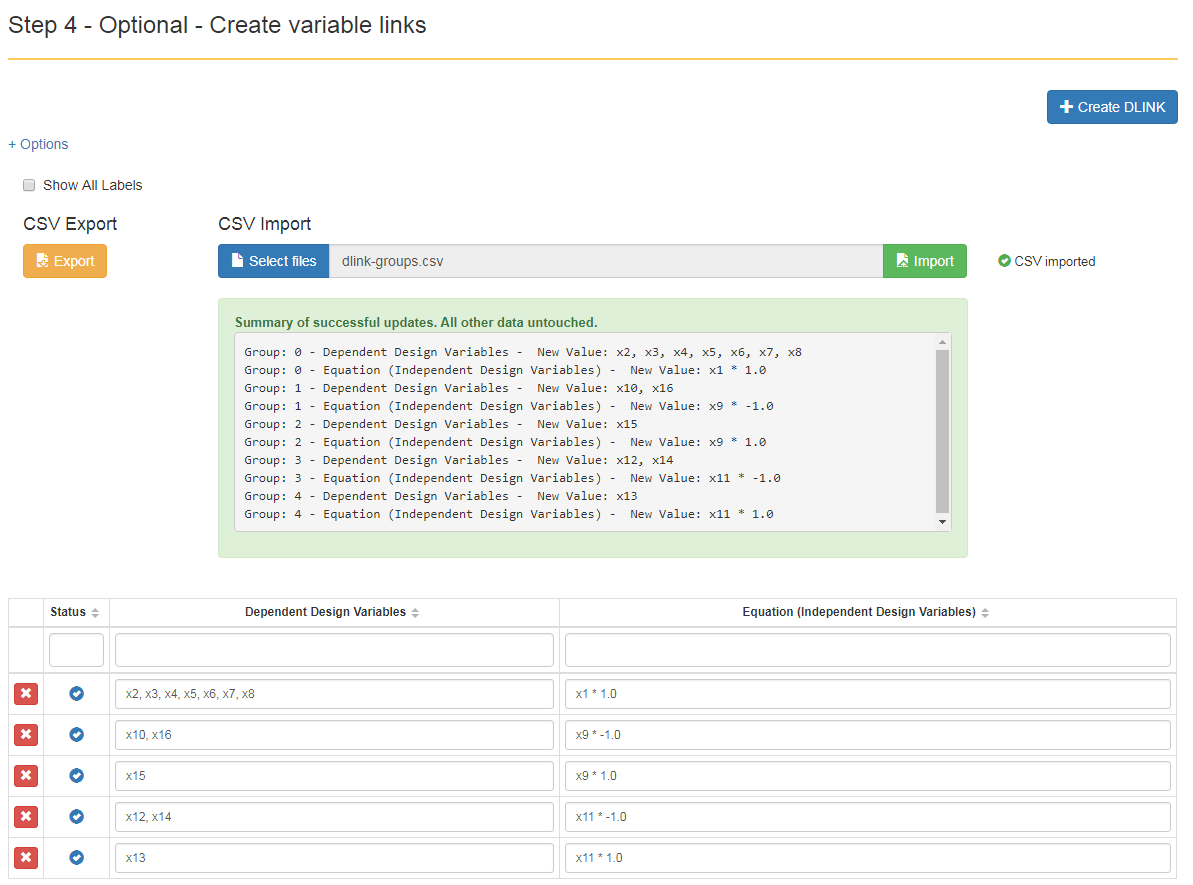
DLINK Support
Before: The previous DLINK implementation was limited to only 1 dependent and 1 independent variable, e.g. x1 = x2 * 1.0. After: The DLINK implementation has been expanded to support linear combinations of independent variables, e.g. x1 = x2 * 1.0 + x3 * -2.0 + x4 * 8.9. This new capability is featured in the tutorial titled Automated Optimization of a Composite Laminate with MSC Nastran Optimization (SOL 200). |
|
|
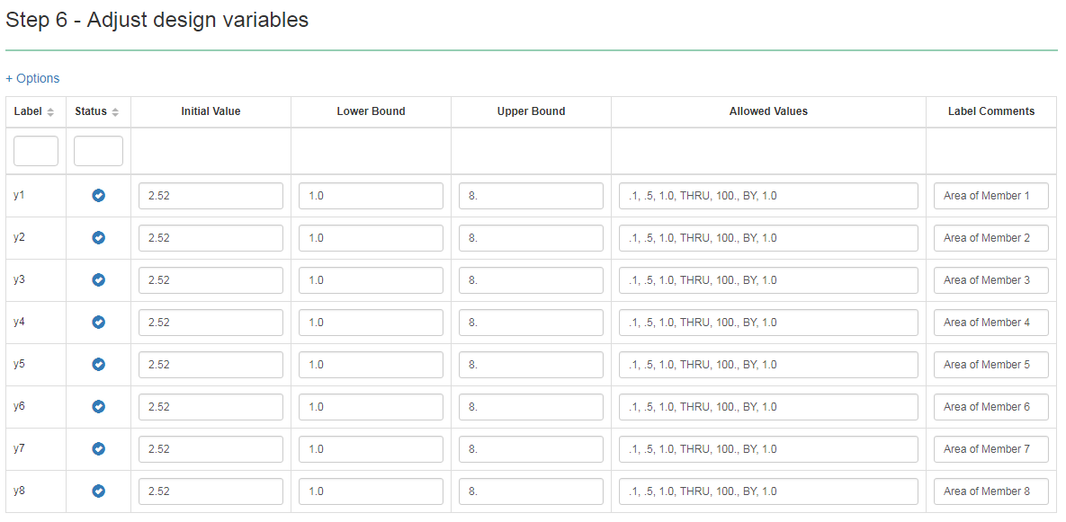
CSV Export/Import for Variables
Before: There was only one method of changing inputs, such as variable bounds and allowed values. This method involved directly changing values on the web page. After: CSV export/import support has been introduced. For variables, a CSV file may be exported, modified in Excel, then imported back to the web app. This speeds up the process of configuring hundreds of variables. This new capability is featured in the tutorial titled CSV Export and Import for Design Variables, Responses and Constraints. |
|
|
CSV Export/Import for Other Responses, Constraints and Equation Constraints (Experimental)
This capability is similar to the existing CSV capability, but differs in the following way. This CSV capability is regarding Other Responses, Constraints and Equation Constraints. This capability is in the experimental stage and will be officially released in a future version. To use this capability, a checkbox titled 'CSV Export/Import (Experimental)' must be marked by going to the Subcase section in the Size Web App. This new capability is featured in the tutorial titled CSV Export and Import for Design Variables, Responses and Constraints. |
|
|
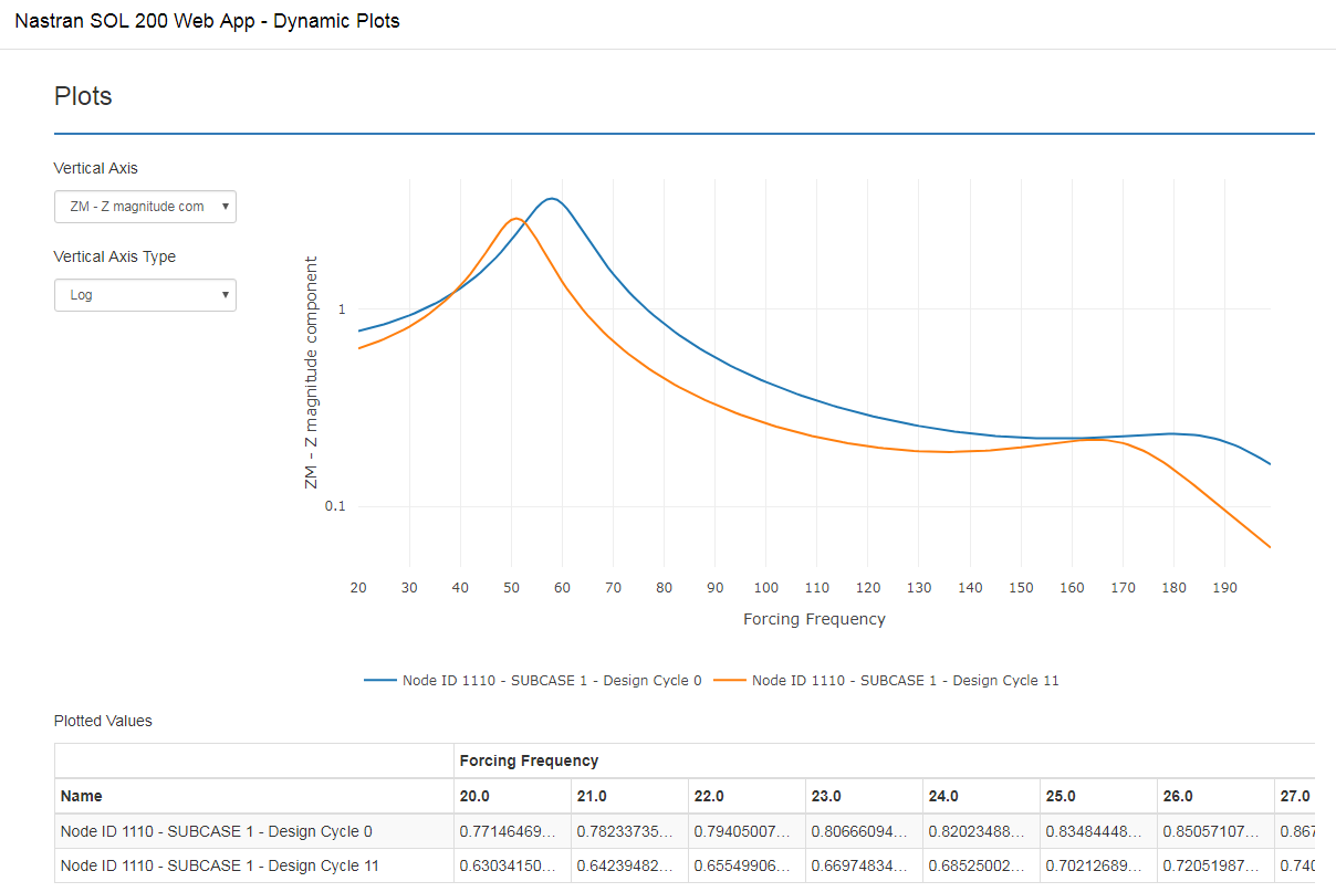
Dynamic Plots
Before: When performing optimization that involves frequency response analysis related to nodal quantities, such as pressure, displacement, velocity, etc., the frequency plots could only be generated outside the web app. After: Such frequency response plots are now automatically generated and displayed. This capability is limited to MSC Nastran 2016 or newer. This new capability is featured in the tutorials titled Dynamic Response Optimization with MSC Nastran Optimization, Acoustic Optimization, Beta Method, and Acoustic Optimization, Nastran BETA Function . |
|
|
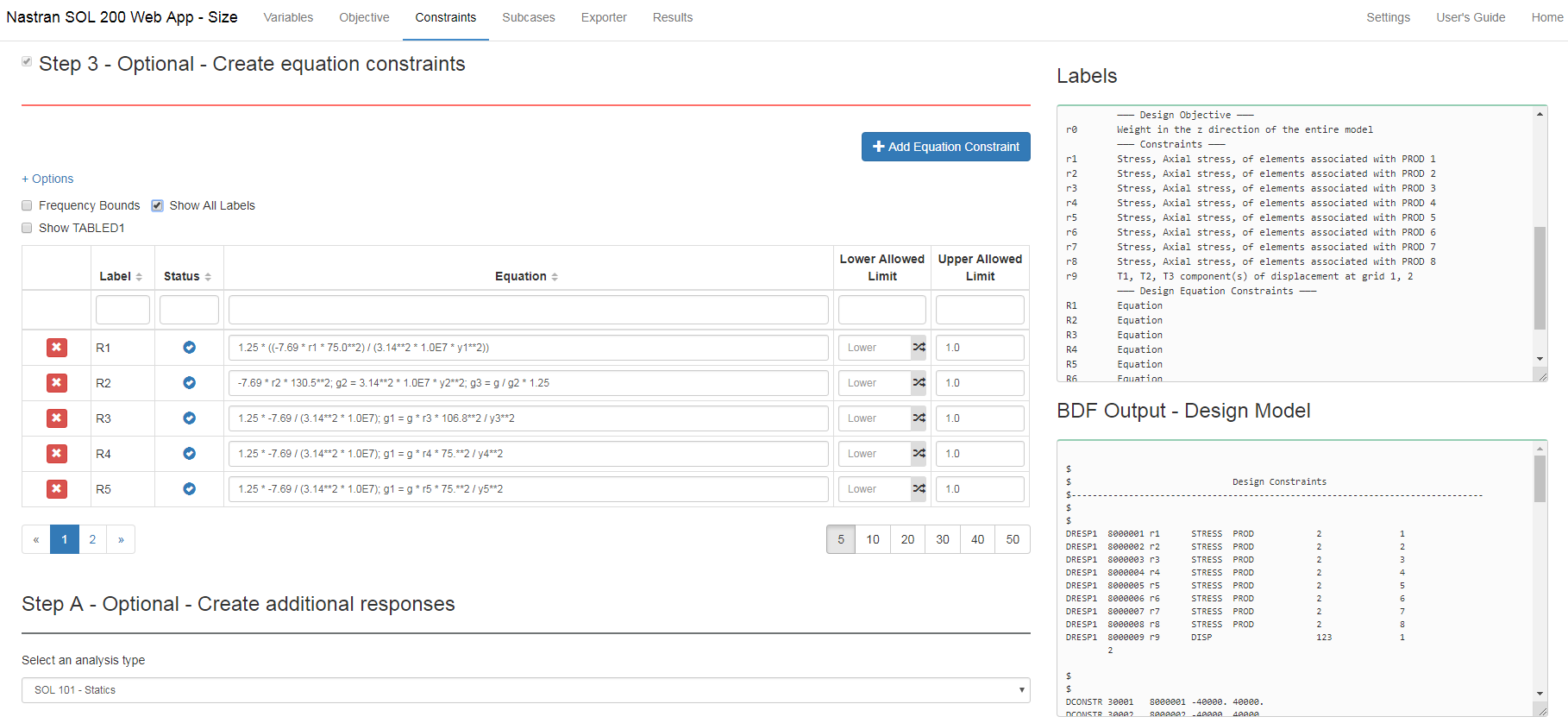
List of Labels in Design Model
Before: Labels are used extensively throughout the web app. The labels are used to define an Equation Objective or Equation Constraints. The labels can be used to generate DLINK entries or assign constraints to Subcases. Previously, the labels could not be simultaneously viewed when creating a definition such as Equation Objective. Excessive navigation was necessary to track and review a label while creating a definition. After: A new option titled 'Show All Labels' has been added to the '+ Options' link. This new option displays all existing labels in a fixed window. When creating a definition, the labels can be viewed in a fixed window without excessive navigation. This new capability is featured in the tutorial titled Optimizing for Buckling - Twenty-Five Bar Truss with MSC Nastran Optimization. |
|
V2.0.0
| New Capabilities and Descriptions | Image of New Capability |
|---|---|
|
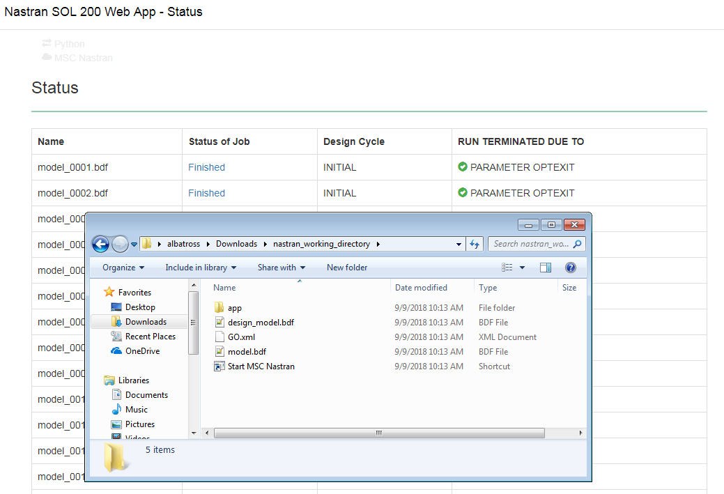
Auto Execute Program
Before: Once BDF files are downloaded from the web app, MSC Nastran must be manually started. Afterwards, the result files, CSV or F06, are to be manually uploaded to the web app. After: A new Auto Execute Program can be downloaded together with the BDF files. This Auto Execute Program will automatically start MSC Nastran, will provide a Status of the optimization, and will automatically upload the optimization results to the web app. This new capability is featured in each Size and Topology workshop. |
|
|
Global Optimization and Parameter Study
Before: MSC Nastran has an existing capability to perform Global Optimization via the MSC Nastran MultiOpt utility. Global Optimization was not previously supported in the Web App. After: Global Optimization can now be configured via the SOL 200 Web App and the Global Optimization results can be displayed. A partial form of Global Optimization, e.g. where only the initial anlaysis is performed for each sample, is also available and is titled Parameter Study. This new capability is featured in the tutorials titled Global Optimization and Parameter Study. |
|
|
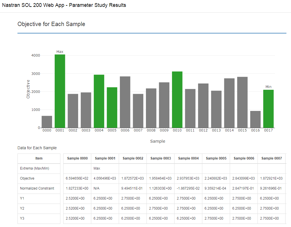
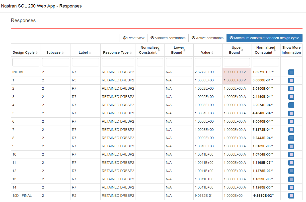
Responses Web App
Before: The F06 file contains explicit information regarding the objective and constraint values for each design cycle. The F06 file in its static text format makes it a challenge to track and review the objective and constraint values. After: A new Responses Web App has been introduced. This web app parses the F06 file for objective and constraint values and summarizes the data in an interactive table. From this table, information regarding the objective or constraints can be quickly queried for each design cycle. This new capability is featured in the tutorial titled Responses in Design Model. |
|
|
CSV for DLINK Entries
Before: There was only one method of configuring DLINK entries. This method involved directly changing values on the web page. After: CSV export/import support has been introduced. For DLINK entries, a CSV file may be exported, modified in Excel, then imported back to the web app. This speeds up the process of configuring hundreds of DLINK entries. This new capability is featured in the tutorial titled CSV Export and Import for Design Variables, Responses and Constraints. |
|
|
Label Comments
Before: The web app uses only two label formats for variables, xi or yi, where i is a positive integer. For design models with hundreds of variables, it became challenging to differentiate numerous variable labels. After: A new input option titled Label Comments is available for labels and allows user to add customized descriptions for each label. |
|
|
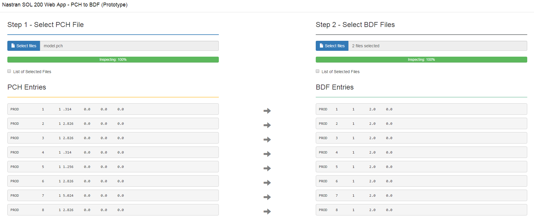
PCH to BDF
Before: After a successful optimization, a PCH file is generated and includes new Bulk Data entries with optimized properties. The final goal is to take the original BDF files and update the Bulk Data entries such that the newest entries from the PCH file are used. This process could only be done via manual text editing or a separate tool outside of the SOL 200 Web App. After: A new web app titled PCH to BDF has been developed and will update existing BDF files with the newest Bulk Data entries found in the .PCH file. This new capability is featured in each Size optimization tutorial. |
|
|
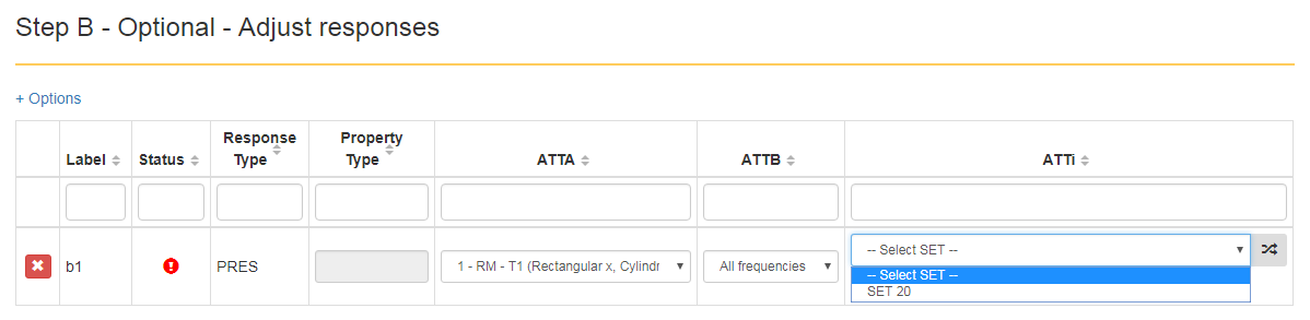
SET ID support
Before: The After: A new option exists in the ATTi input boxes that allows the selection of existing SETs and its respective list of IDs are automatically inserted into the ATTi input box. This makes selection of specific IDs faster when defining constraints or other responses. |
|
Connected Clients
What is design optimization?
Before describing design optimization, it is best to first define optimization and present a brief mathematical example.
Optimization is the process of finding a minimum or maximum to a given objective function and constraints.
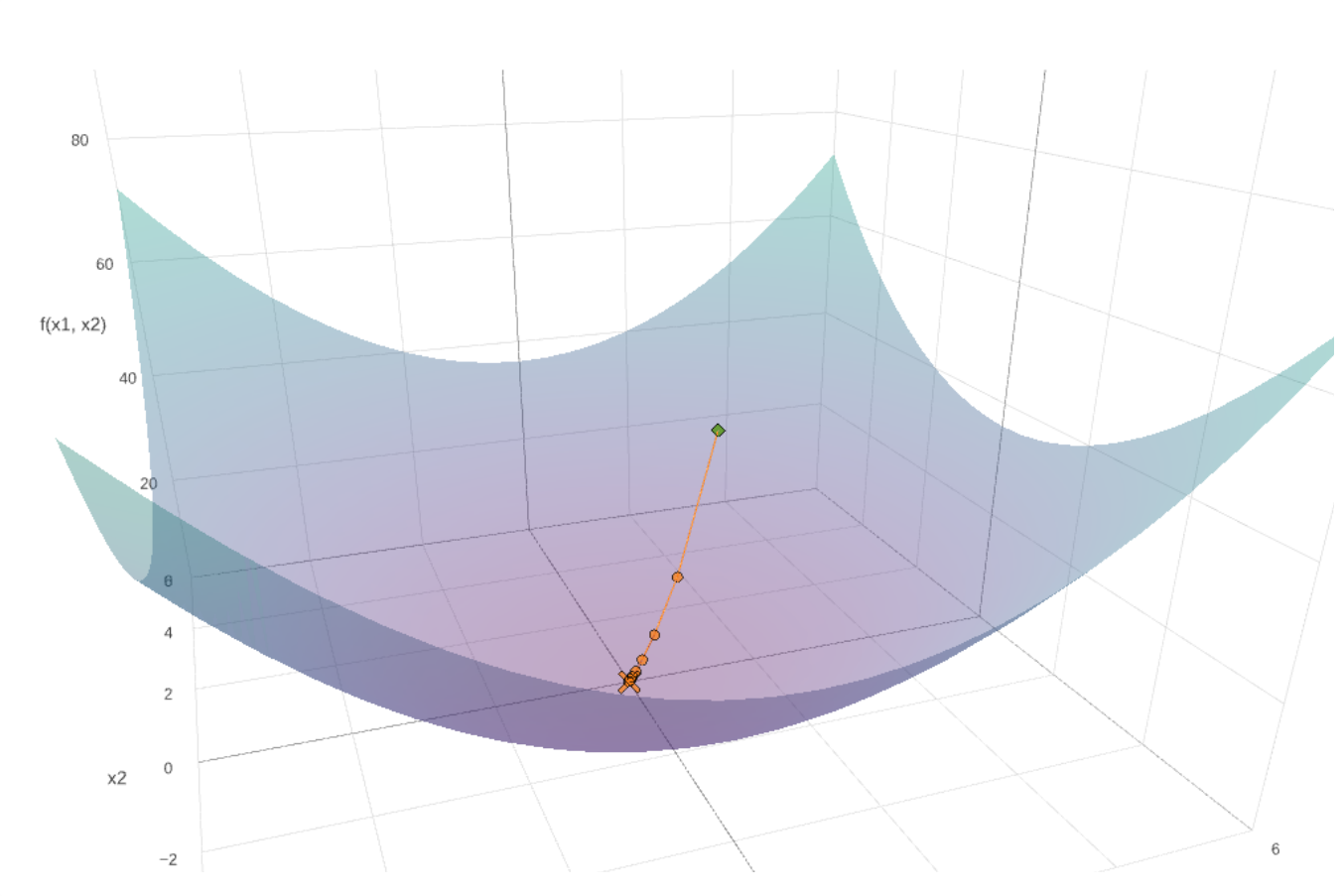
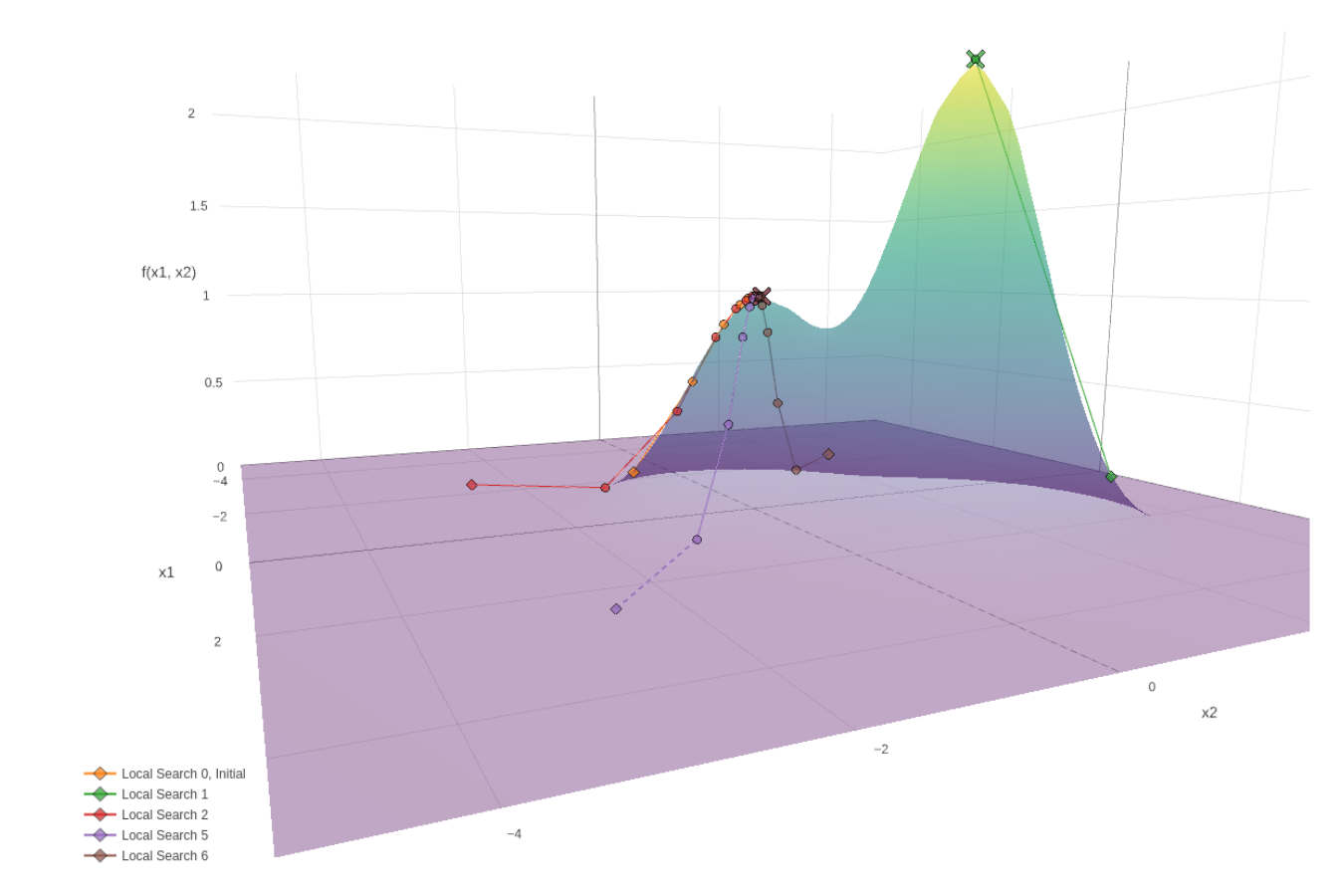
Consider this objective function.
The objective function's surface plot is shown in Figure 1. The problem posed is to find the minimum of the objective function given that the starting or initial point is (x1, x2) = (3, 4) . This example can easily be done by hand. Alternatively, an optimizer, such as the one available in MSC Nastran SOL 200, can be used to automatically search for the minimum. Figure 1 shows the search path the SOL 200 optimizer took to find the minimum.
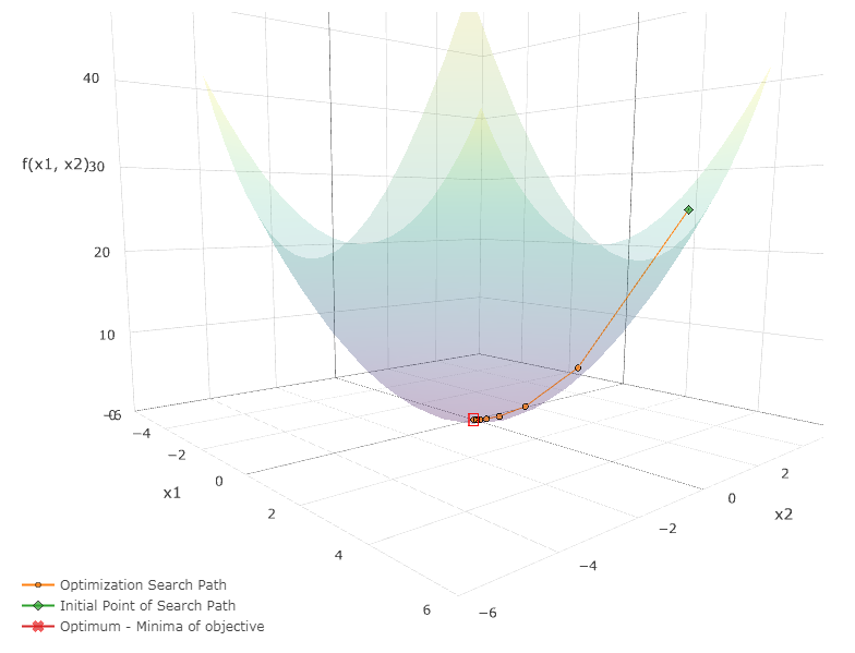
Figure 1
Design optimization is essentially regular optimization, i.e. the goal is to find a minimum or maximum of an objective function, but is different in the sense that now a structural model is being optimized. Objectives are expressed as minimizing the weight, maximizing the stiffness of a structure, or finding the optimum of some other response or quantity. If performing size optimization, variables such as x1, x2 are now corresponding to structural parameters such as plate thickness or dimensions of beam cross sections. Constraints are limits imposed on stress, displacement, or many other types of structural responses.
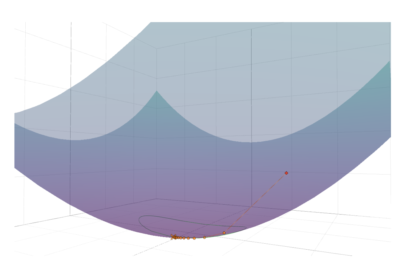
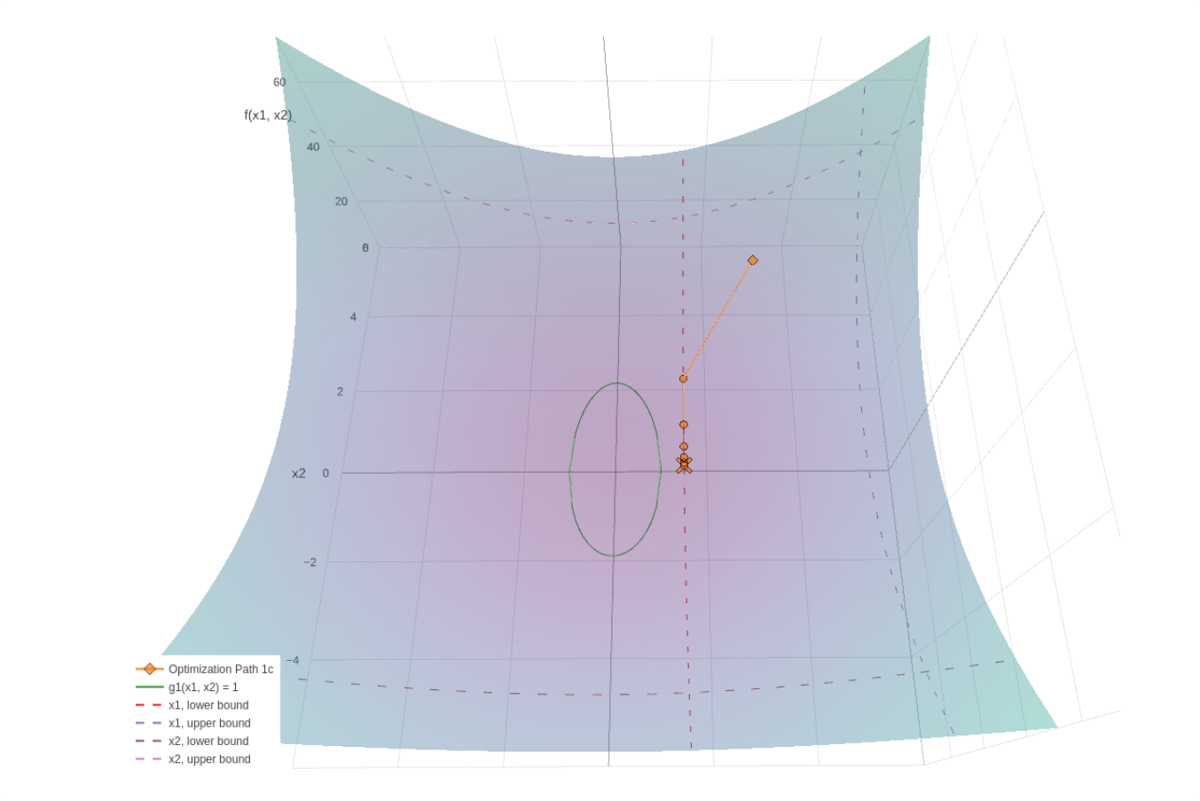
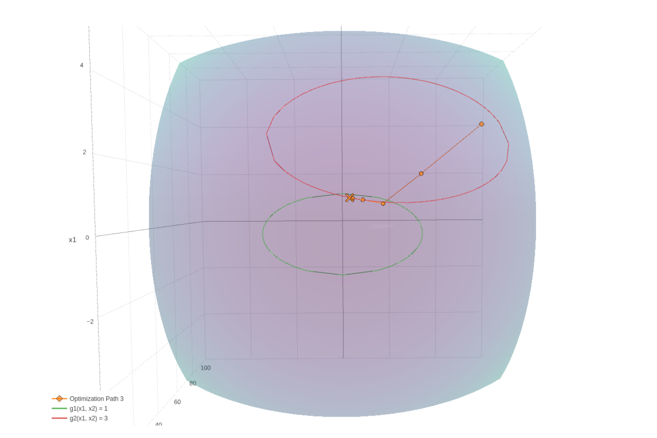
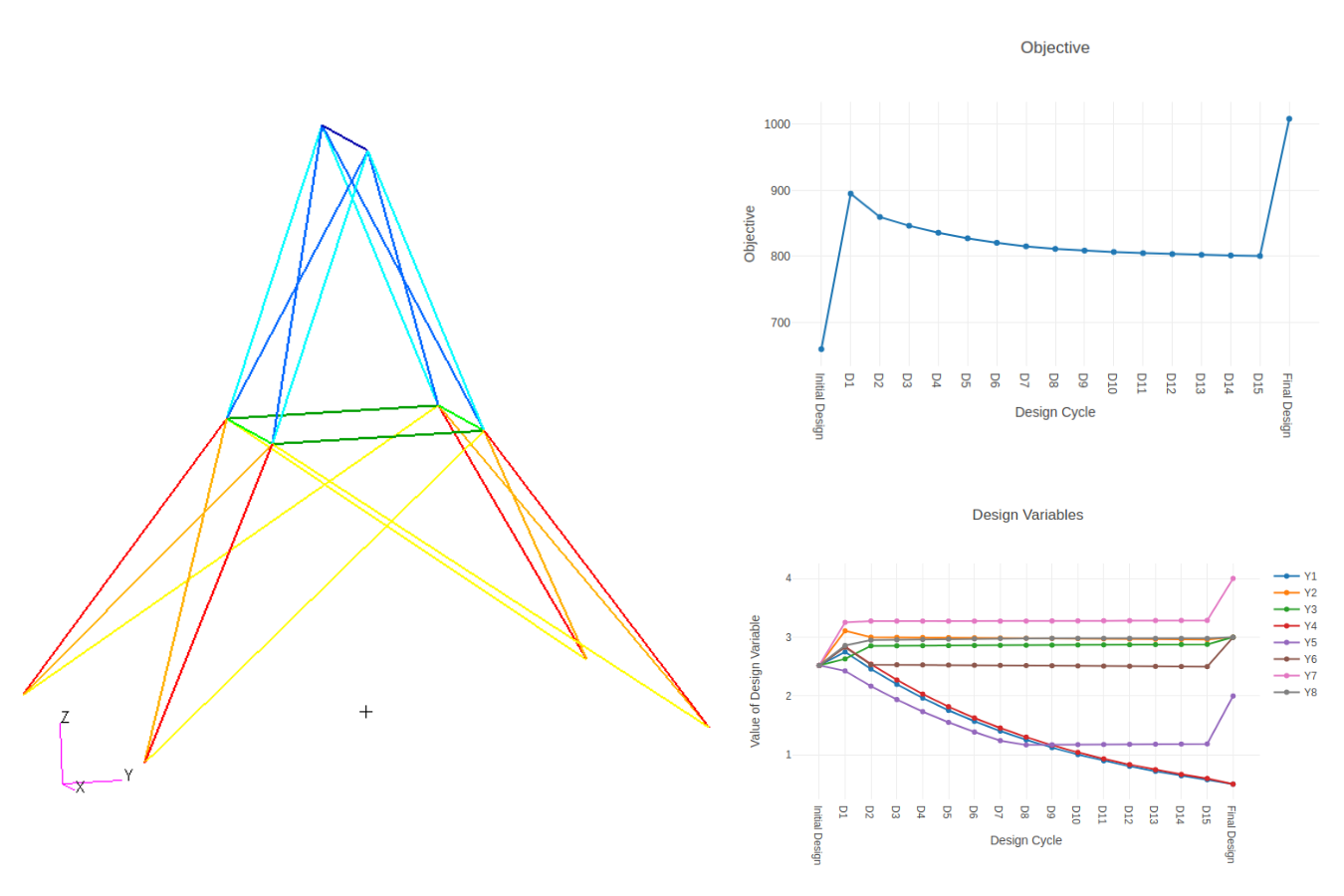
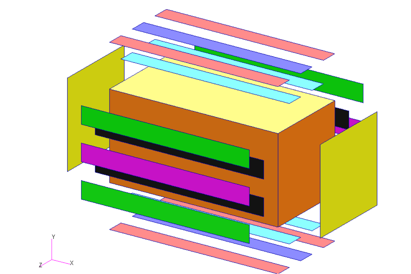
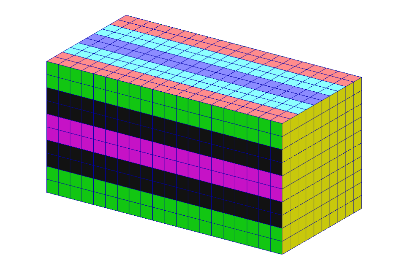
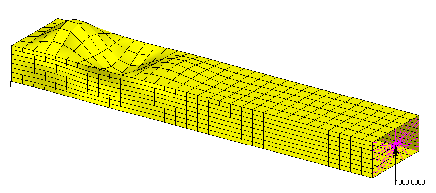
Consider the following design optimization example, Figure 2, from the MSC Nastran Design Sensitivity and Optimization User's Guide. Like regular optimization, an objective, constraints and design variables are specified, but are directly associated with a structural model.

Figure 2
This example has two design variables, and the result of the MSC Nastran Optimization can be plotted three dimensionally. See Figure 3.
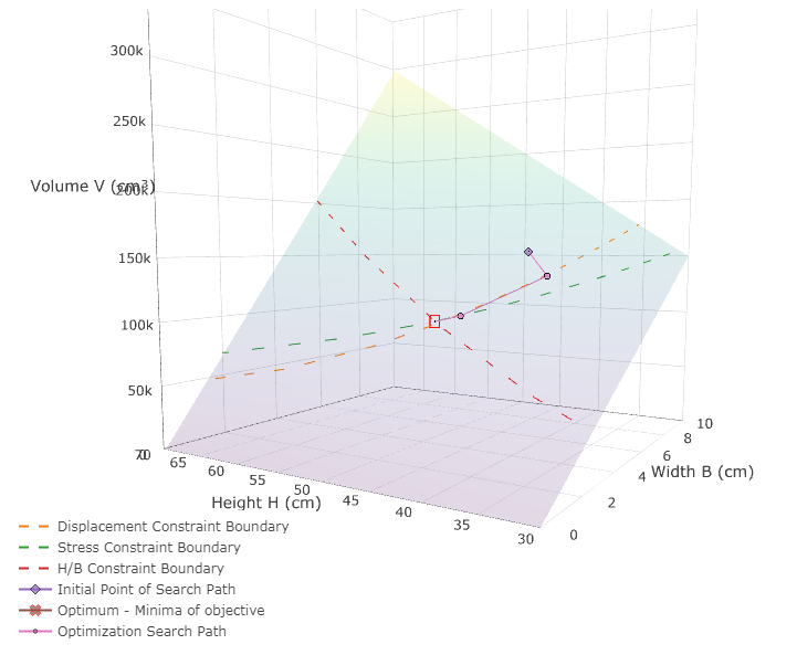
Figure 3
Table 1 compares optimization and design optimization. As can be seen, both are very similar, except that with design optimization the objective, variables and constraints are associated with a structural model.
Table 1
| Optimization | Design Optimization | |
|---|---|---|
| Objective | Minimize f(x1, x2) = x12 + x22 | Minimize volume of structure |
| Constraints | g(x1, x2) = x12 + (x2 / 2)2 g < 20000 |
σ < 700 δ < 2.54 |
| Variables | x1 x2 |
B: Width H: Height |
Description of MSC Nastran Design Sensitivity and Optimization
The optimization capability available in MSC Nastran SOL 200 is quite extensive and offers engineers multiple methods to improve structural designs.
For example, design sensitivity analysis is the process of computing partial derivatives or sensitivities of structural responses with respect to design variables. These sensitivities can be used to determine which design variables will have the most impact on achieving a desired objective. Design optimization is the actual process of determining an optimum configuration of a finite element model to achieve a minimum or maximum objective. During the optimization process, optimizers are constantly computing sensitivities to determine the best search paths to take in order to find minimums or maximums.
For a brief introduction to MSC Nastran SOL 200, please refer to the Introduction to Nastran SOL 200 Design Sensitivity and Optimization eBook.
A comprehensive list of each optimization feature is available in the MSC Nastran Design Sensitivity and Optimization User's Guide.
SOL 200 Web App
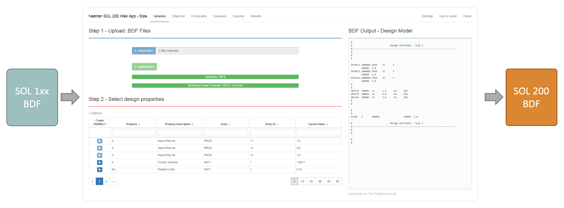
To use MSC Nastran SOL 200, an existing SOL 1xx BDF file must be converted to SOL 200. The conversion process involves the selection of design variables, objective, and constraints. The SOL 200 Web App, web app for short, facilitates the conversion process. The Supported Capabilities section of this guide details what the web app supports in MSC Nastran SOL 200.
Apps
Converter
The Converter App takes existing SOL 200 BDF files and ensures each SOL 200 bulk data entry is in a compatible format.The SOL 200 Web App (web app) uses a specific set of identification numbers (IDs) and labels (LABELs) for each bulk data entry. For example, the DESVAR entry created by the web app will either have an ID starting at 100001 or 200001 and labels xi or yi, where i is a positive integer. Bulk data entries not using specific IDs or LABELs are not recognized by the web app. As a result, BDF files with SOL 200 entries, e.g. DESVAR, DRESP1, etc., created by other tools cannot be uploaded to the web app without first converting the BDF files.
Supported Entries
The following bulk data entries can be converted. All other bulk data entries not listed are not supported.- BEADVAR
- DCONADD
- DCONSTR
- DDVAL
- DEQATN
- DESVAR
- DLINK
- DRESP1
- DRESP2
- DVPREL1, DVMREL1, DVCREL1
- DVPREL2, DVMREL2, DVCREL2
- TOMVAR
- TOPVAR
Modified Fields
The goal of the conversion process it to update each entry such that the entry ID and LABEL are compatible with the web app. All other fields are left untouched.For example, the entry below is changed as follows. The ID in Field 2 is updated. The LABEL in Field 3 is updated. All other fields, Fields 1, 4, 5, 6 and 7, are left untouched.
$   1  ||   2  ||   3  ||   4  ||   5  ||   6  ||   7  ||   8  |
DESVAR  1       A1      .8365   .1      100.    1.
$   1  ||   2  ||   3  ||   4  ||   5  ||   6  ||   7  ||   8  |
DESVAR  1       A1      .8365   .1      100.    1.
Converting to Equivalent Entries
There are multiple ways to express the same configuration. For example, suppose the design variables y10, y20 and y30 exist and the goal is to relate the thickness T as follows:T = y10 * 1.0 + y20 * 1.000 + y30 * 1.0 + .5
Consider the Original Entry and Equivalent Entries below. The Original Entry expresses this relationship.
On the DVPREL1 entry, the SOL 200 Web App does not support fields 8, 13, 14, 15, etc. An equivalent set of entries is instead created during conversion to match the same configuration. See the Equivalent Entries..
DVPREL1 1       PSHELL  1       T                       .5
        10      1.0     20      1.000   30      1.0
DVPREL2 2000001 PSHELL  1       T                       5001
DESVAR  200010  200020  200030
DEQATN  5001
        g(y10,y20,y30) =
        y10 * 1.0 + y20 * 1.000 + y30 * 1.0 + .5
DVPREL1     402 PBRSECT 11994   T
              2 1.000
DVPREL1     403 PBRSECT 11994   T(1)
              2 1.000
DESVAR        2 T11994  1.000   0.600   8.000
DVPREL1 1000402 PBRSECT 11994   T
         100402 1.000
DVPREL1 1000403 PBRSECT 11994   T(1)
         100403 1.000
DESVAR   100402 x402    1.000   0.600   8.000
DESVAR   100403 x403    1.000   0.600   8.000
DLINK   1       100403                  100403  1.0
DRESP2  30005   RTSUMSQ MAX
DRESP1  10001   10002   10003   10004   10005   10006   10007
DRESP2  9030005 R30005  170005
DRESP1  7010001 7010002 7010003 7010004 7010005 7010006 7010007
DEQATN  170005
        g(b10001,b10002,b10003,b10004,b10005,b10006,b10007) =
        MAX(b10001,b10002,b10003,b10004,b10005,b10006,b10007)
Solution Discrepancies
For most cases, the converted version of the BDF files will produce an optimization solution identical to the original BDF files. There have been a small number of instances where slight differences of less than one percent(1%) in the solutions have been observed. The goal in this section is to document reasons the slight differences occur.The .dat files referenced are found in the Test Problem Library (TPL), a folder included in the MSC Nastran Documentation installation directory.
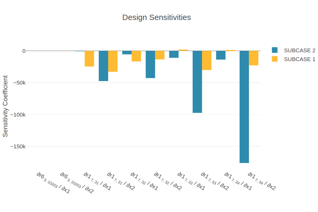
- For file dsoug3.dat, the DVPREL1 entries are converted to DVPREL2 entries. This change has implications when the sensitivity coefficients are computed.
- For file dsoug7.dat, the DVPREL1 entry is using PMIN. The web app does not support the PMIN or PMAX fields and will remove the PMIN or PMAX fields. The limits are already specified on the DESVAR entry and renders the use of PMIN or PMAX unnecessary.
- For file dsoug8.dat, the DEQATN entry uses PI(1) to signify the value of 3.14. The Converter App replaces PI(1) with 3.1416. PI(1) is not supported by the web app.
- For file dsoug14.dat, the original DESVAR entry is in the large field format. The initial value of the original DESVAR entry is 8.36519659E-01, but after conversion, the entry uses the small field format. As a result, the new initial value is .8365. The web app creates entries only in the small field format.
Tutorials
Over 25 step-by-step tutorials are available regarding fundamentals of optimization and how to properly use the SOL 200 Web App. Click on any of the following links to jump to the section.
- Optimization Basics
- Size Optimization Tutorials
- Topology, Topometry and Topography Tutorials
- Advanced Tutorials
- Miscellaneous Tutorials
- Machine Learning Tutorials
- Beams Tutorials
- Composite Laminate Optimization Tutorials
- Shape Optimization Tutorials
- Post-processor Tutorials
- Uncertainty Quantification Tutorials
- Optimization Under Uncertainty Tutorials
Optimization Basics
| Title and Description | YouTube Tutorial | |
|---|---|---|
 |
Unconstrained Optimization with MSC Nastran SOL 200 Part of Calculus involves finding maximums or minimums of functions. The process of finding maximums or minimums is the essence of optimization. In this video, MSC Nastran Optimization is used to find the optimum point or minimum of a two-variable function, f(y1, y2) = y1^2 + y2^2. |
Link |
 |
Constrained Optimization with MSC Nastran SOL 200 This video demonstrates the use of MSC Nastran Optimization to find the minimum of f(y1, y2) subject to a constraint g(y1, y2). |
Link |
 |
Side Constraints on Design Variables - MSC Nastran Optimization This video demonstrates the use of MSC Nastran Optimization to find the minimum of f(y1, y2) subject to limits on the design variables y1 and y2. |
Link |
 |
Best Compromise Infeasible Design - MSC Nastran Optimization In constrained optimization, an optimum solution may not exist that satisfies all the constraints. This video demonstrates such a scenario and walks through a fix. |
Link |
 |
What is Global Optimization? MSC Nastran SOL 200 / Optimization Tutorial This video discusses the meaning of Global Optimization and walks you through the process of setting up a Global Optimization with MSC Nastran SOL 200. |
Link |
 |
What is size optimization? What is shape, topology, topography and topometry optimization? In this short video, the following MSC Nastran optimization types are described.
|
Link |
Size Optimization Tutorials
| Title and Description | Lecture Notes | PDF Tutorial | YouTube Tutorial | |
|---|---|---|---|---|
 |
Structural Optimization of a 3 Bar Truss - MSC Nastran Optimization A truss structure is optimized with MSC Nastran. The design variables are the cross-sectional areas of the rod elements. The objective is to minimize the weight of the structure while ensuring the stress and displacements are within specified constraints. Starting BDF Files: Link Solution BDF Files: Link |
Link | Link | Link |
 |
Sensitivity Analysis of a 3 Bar Truss - MSC Nastran Optimization A structural optimization was previously performed on a 3 bar truss. In this tutorial, the process to perform a sensitivity analysis is detailed. Starting BDF Files: Link Solution BDF Files: Link |
Link | Link | |
 |
Automated Structural Optimization of a Stiffened Plate with MSC Nastran SOL 200/Design Optimization This example demonstrates the use of MSC Nastran to optimize the thickness of the plate and the thickness of a beam section to minimize weight. Constraints are imposed on the stresses in the shell and beam elements. Additional constraints are imposed on deflections. Starting BDF Files: Link Solution BDF Files: Link |
Link | Link | Link |
 |
Vibration of a Cantilevered Beam (Turner's Problem), MSC Nastran Optimization This example demonstrates the use of MSC Nastran to optimize the rod areas and shell thicknesses such that the structure's weight is minimized and the first natural frequency is above 20 Hz. Starting BDF Files: Link Solution BDF Files: Link |
Link | Link | Link |
 |
Dynamic Response Optimization with MSC Nastran Optimization This example is from the MSC Nastran Design Sensitivity and Optimization User's Guide. Starting BDF Files: Link Solution BDF Files: Link |
Link | Link | Link |
 |
Model Matching, Frequency Response Analysis A frequency response analysis has been performed, but the results do not match experimental results. This tutorial discusses the model matching procedure in order to correlate Finite Element Analysis and test results. Starting BDF Files: Link Solution BDF Files: Link |
Link | Link | |
 |
Using MSC Nastran Optimization for Model Matching / System Identification In this example, the cross section of a rod is designed such that the analysis modes match experimentally measured data. MSC Nastran Optimization is used to minimize the root sum of squares for Mode 1. This example is an adaptation of the example found in the UAI/Nastran User's Guide for Version 20.1 - 252.6.6 System Identification. The following is an excerpt from the guide describing this example. Keep in mind this video is an adaptation and will not match all the values in the following description: Starting BDF Files: Link Solution BDF Files: Link |
Link | Link | Link |
 |
Ply Number Optimization of a Composite Laminate with MSC Nastran Optimization (SOL 200) This tutorial details the process to configure a ply number optimization for MSC Nastran. The optimization problem statement is to reduce the mass of a composite cylinder, ensure ply failure index constraints are satisfied, and vary the number of plies for 0, 90 and +/-45-degree layers. This example considers ply number optimization for multiple PCOMP entries and multiple load cases. Additional comments are made regarding displaying fringe plots of the failure indices after optimization, updating the final BDF files with new PCOMP entries, and stacking sequence optimization. Starting BDF Files: Link Solution BDF Files: Link |
Link | Link | |
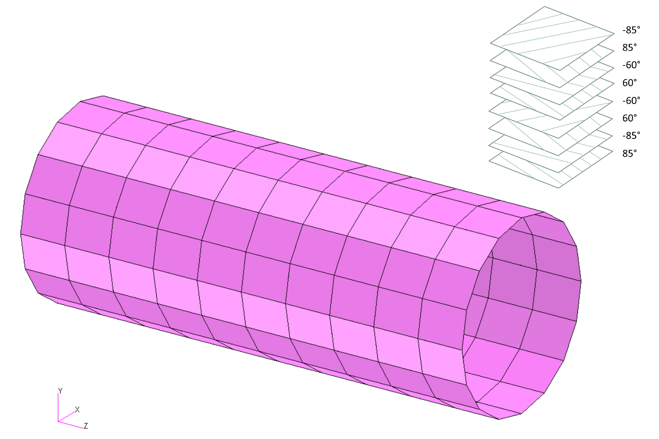 |
Automated Optimization of a Composite Laminate with MSC Nastran Optimization (SOL 200) This example details the use of MSC Nastran Design Optimization (SOL 200) to optimize the weight of a tube composed of a composite laminate. The ply thicknesses and orientations are allowed to vary during the optimization process. The orientation angles are limited to 5 degree increments. Constraints on the failure indices are applied. Starting BDF Files: Link Solution BDF Files: Link |
Link | Link | Link |
 |
Optimizing for Buckling - Twenty-Five Bar Truss with MSC Nastran Optimization This example is from the MSC Nastran Design Sensitivity and Optimization User's Guide.
Starting BDF Files: Link Solution BDF Files: Link |
Link | Link | Link |
 |
Acoustic Optimization, Beta Method A fluid is enclosed in a structural box and subjected to an acoustic source. The goal is to minimize the peak acoustic pressure while letting the structural thicknesses vary and preventing the weight from significantly changing. Starting BDF Files: Link Solution BDF Files: Link |
Link | Link | Link |
 |
Acoustic Optimization, Nastran BETA Function This tutorial is a repeat of the previous Acoustic Optimization example, but highlights an alternative method to setting up the optimization for Nastran SOL 200. The BETA method is used and reduces the work that was previously required. Starting BDF Files: Link Solution BDF Files: Link |
Link | Link | |
 |
Optimization for Multiple Load Cases or SUBCASEs The web app makes simple configuring design constraints for dozens or hundreds of load cases. This tutorial guides you through the process. Starting BDF Files: Link Solution BDF Files: Link |
Link | Link | |
 |
Buckling Optimization of a Cantilever Beam This example demonstrates the procedure to configure Nastran SOL 200 for buckling optimization. This example also covers how to optimize for multiple buckling scenarios. Starting BDF Files: Link Solution BDF Files: Link |
Link | Link | |
|
Global Optimization This example demonstrates the procedure of performing a Global Optimization with MSC Nastran SOL 200. Often, optimization problems have multiple local minimums, or maximums, when starting from different initial design variables. To find the global optimum, multiple local optimizations must be performed, then the best of the local optimizations is taken to be global optimum. This process can be performed with the Global Optimization capability available in MSC Nastran SOL 200. Starting BDF Files: Link Solution BDF Files: Link |
Link | Link | |
|
Parameter Study This tutorial details the use of MSC Nastran SOL 200 to perform a "parameter study." What is a parameter study? A common engineering technique is to try different structural configurations, for example, changing structural dimensions, and review the impact on structural responses such as displacements and stresses. Dozens, possibly hundreds of structural configurations would ideally be evaluated. This is termed "parameter study." MSC Nastran SOL 200 includes a capability to automatically generate multiple structural configurations and perform static or dynamic analyses. The outcome are results from multiple structural configurations that can be compared. Starting BDF Files: Link Solution BDF Files: Link |
Link | Link | |
 |
Multi Model Optimization Multi Model Optimization (MMO) is the process of optimizing multiple design models concurrently. Design variables across multiple models can be linked and simultaneously optimized. A merged or combined objective can optimize the objective of each design model. The design constraints of each design model are also included in a multi model optimization. This tutorial details the procedure to configure a multi model optimization. Starting BDF Files: Link Solution BDF Files: Link |
Link | Link |
Topology, Topometry and Topography Tutorials
| Title and Description | Lecture Notes | PDF Tutorial | YouTube Tutorial | |
|---|---|---|---|---|
 |
MSC Nastran Topology Optimization - Minimizing mass with stress and displacement constraints A solid block of material composed of 3D or Hexahedral elements is subjected to two load cases. Topology Optimization is used to minimize the mass of the structure, while satisfying both stress and displacement design constraints. Starting BDF Files: Link Solution BDF Files: Link |
Link | Link | Link |
 |
MSC Nastran Topology Optimization Manufacturing Constraints A cantilever beam is composed of 3D or Hexahedral elements and a load is applied at the free end. Topology Optimization is used to identify regions of material to remove. This example discusses options to produce a symmetric design and a design that can be manufactured via casting. Starting BDF Files: Link Solution BDF Files: Link |
Link | Link | Link |
 |
MSC Nastran Topology Optimization Mirror Symmetry Constraints A plate composed of 2D finite elements, is simply supported and has a load applied at the midpoint. Topology Optimization is used to identify material to remove. This example focuses on satisfying weight, stiffness and symmetry targets. Starting BDF Files: Link Solution BDF Files: Link |
Link | Link | Link |
 |
MSC Nastran Topology Optimization - Multidiscipline - Static Loading and Natural Frequency A simply supported plate is composed of 2D finite elements and a load is applied at the midspan. The MSC Nastran Topology Optimization capability is used to determine which portions of the plate should be kept while satisfying weight, stiffness and first natural frequency constraints. This example also showcases the ability to optimize for multiple analysis types, e.g. static and normal modes analysis. Starting BDF Files: Link Solution BDF Files: Link |
Link | Link | Link |
 |
MSC Nastran Topometry Optimization of a Cantilever Plate This tutorial is an introduction to Topometry Optimization. A simple cantilever plate is used to demonstrate element-by-element optimization of thickness. Starting BDF Files: Link Solution BDF Files: Link |
Link | Link | Link |
 |
MSC Nastran Topometry Optimization with Symmetry Constraints This tutorial details the configuration of symmetry constraints in a topometry optimization. Starting BDF Files: Link Solution BDF Files: Link |
Link | ||
 |
MSC Nastran Topography Optimization - Bead or Stamp Optimization This tutorial covers the use of Topography Optimization to determine optimal bead or stamp patterns. The Post-processor web app is used afterwards to review the results of the optimization. Starting BDF Files: Link Solution BDF Files: Link |
Link |
Advanced Tutorials
| Title and Description | PDF Tutorial | YouTube Tutorial |
|---|---|---|
| Manually Starting MSC Nastran and Uploading Results This tutorial discusses how to manually start MSC Nastran. This tutorial also discusses how to upload result files (.f06, .csv or multiopt.log) to the SOL 200 Web App. | Link | Link |
| CSV Export and Import for Design Variables, Responses and Constraints Large design models may have thousands of design variables and constraints. The web app supports the export and import of CSV files. With the aid of Excel, hundreds of entries can be rapidly configured. This tutorial discusses the CSV export and import functionality. | Link | |
| Responses in Design Model Responses are the outputs following a structural analysis. Some examples include displacements at nodes, stresses in elements, etc. Each design cycle during the optimization process involves a structural analysis and the production of responses. This tutorial discuses the use of the Responses App to carefully inspect responses found in the .f06 file. | Link | |
| The Design Cycle Process of MSC Nastran SOL 200/Optimization MSC Nastran Optimization or SOL 200 takes multiple design cycles to shift the design variable values, for example dimensions of your structure, until an optimum of your objective is reached. This video walks you through the design cycle process in MSC Nastran Optimization. |
Link | |
| Summary of Design Cycle History in the .f06 file - MSC Nastran Optimization At the end of an optimization with MSC Nastran, the final summary of the optimization is available at the bottom of the .f06 file. This video discusses how to interpret the final summary. |
Link | |
| Viewing Optimization results in Excel - MSC Nastran Optimization The results of an MSC Nastran Optimization can be viewed in excel. Information such as the change of objective and design variables can be viewed for each design cycle. This video walks you through the process of viewing optimization results in excel. |
Link | |
| How to create a new bdf file with optimized properties - MSC Nastran Optimization Once MSC Nastran Optimization has produced optimized design variables, e.g. optimized structural dimensions, the original .bdf/.dat file must be updated with the new property values. This video establishes two methods of updating the original .bdf/.dat file. |
Link | |
| How to fix 'RUN TERMINATED DUE TO HARD CONVERGENCE TO A BEST COMPROMISE INFEASIBLE DESIGN' MSC Nastran SOL 200 or Design Optimization employs an intelligent method of handling hundreds of design constraints. This video covers the following:
|
Link | |
| How to perform a Sensitivity Analysis in MSC Nastran SOL 200 This video details 3 methods of performing a sensitivity analysis with MSC Nastran. The following points are discussed: What is sensitivity analysis? How to perform a sensitivity analysis with MSC Nastran Interpreting the sensitivities |
Link | |
| How to verify design variables - MSC Nastran Optimization Configuring a design model for MSC Nastran Optimization is a simple process, but care must be taken to ensure the configuration was properly done. This video details how to verify that design variables have been properly configured. |
Link | |
| How to verify design constraints - MSC Nastran Optimization A simulation of a Finite Element model can produce an overwhelming amount of output such as displacements, stresses, strain, etc. Design constraints are imposed on specific outputs. This video outlines a procedure to ensure the design constraints are applied to the correct responses such as displacements, stresses, strains, etc. |
Link |
Miscellaneous Tutorials
| Title and Description | PDF Tutorial | YouTube Tutorial | |
|---|---|---|---|
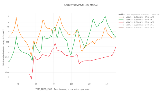 |
Use the HDF5 Explorer to Create Plots Starting with MSC Nastran 2016, results can be outputted to the HDF5 file type. This tutorial introduces the HDF5 Explorer and the following concepts:
|
Link | |
|
Remote execution of MSC Nastran on a remote operating system available on the local network This tutorial discusses the use of the Remote Execution web app and how to run MSC Nastran jobs on remote operating systems available on the local network. Traditionally, FTP and SSH programs are required to run MSC Nastran on remote operating systems, but this tutorial discusses how to run MSC Nastran through the web browser alone. FTP and SSH programs are not required for this tutorial. |
Link | |
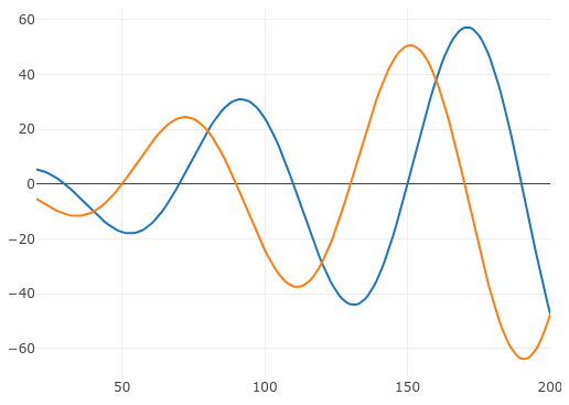 |
Creation of Dynamic Loads via RLOAD1 or RLOAD2 Entries A critical part of dynamic analysis is defining the dynamic load. For frequency response analysis, the dynamic load is defined via the RLOAD1 or RLOAD2 bulk data entries. For the simplest dynamic loads, only RLOAD1 or RLOAD2 entries are sufficient. For more complex dynamic loads, the following entries might be required: RLOAD1, RLOAD2, TABLED1, TABLED2, TABLED3, TABLED4, DELAY or DPHASE. This exercise details the use of the Dynamic Loads web app to define dynamic loads and the following entries: RLOAD1, RLOAD2, TABLED1, TABLED2, TABLED3, TABLED4, DELAY or DPHASE. Starting Files: Link Solution BDF Files: Link |
Link | |
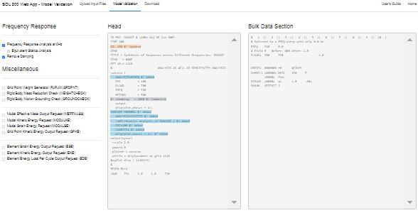 |
Configure a 0 Hz Frequency Response and Statics Analysis One recommended strategy when configuring a frequency response analysis is the following: Perform a frequency response analysis at 0 Hz and a statics analysis. If the results of both analyses are significantly different, there may be an issue that needs to be addressed. This exercise details the use of the Model Validation web app to configure a 0 Hz frequency response and statics analysis. A comparison of the results is also done. Ultimately, the results are identical and confirms there are no unintended issues in the model. Starting BDF Files: Link Solution BDF Files: Link |
Link |
Machine Learning Tutorials
| Title and Description | PDF Tutorial | YouTube Tutorial | |
|---|---|---|---|
|
Introduction - MSC Nastran Machine Learning Web App There are many machine learning methods available, such as neural networks, decision trees, genetic algorithms, supervised learning, etc. Watch this presentation to gain an understanding of the machine learning methods implemented in the MSC Nastran Machine Learning web app. The MSC Nastran Machine Learning web app makes use of the following methods:
|
Link | Link |
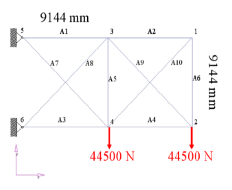 |
Machine Learning, Structural Optimization of a 10 Bar Truss with MSC Nastran SOL 400 Machine learning methods are used to optimize a truss structure. This example features the optimization of nonlinear responses from MSC Nastran SOL 400. MSC Nastran is used to evaluate the FE model. The design variables are the cross-sectional areas of the rod elements. The objective is to minimize the weight of the structure while constraining the axial stresses and displacements. Most machine learning examples are lower dimension problems with 1 to 5 parameters. This tutorial demonstrates a higher dimension scenario with 10 parameters. Starting Files: Link Solution BDF Files: Link |
Link | Link |
|
Machine Learning, Structural Optimization of a 3 Bar Truss Machine learning methods are used to optimize a truss structure. MSC Nastran is used to evaluate the FE model. The design variables are the cross-sectional areas of the rod elements. The objective is to minimize the weight of the structure while constraining the axial stresses. Starting Files: Link Solution BDF Files: Link |
Link | Link |
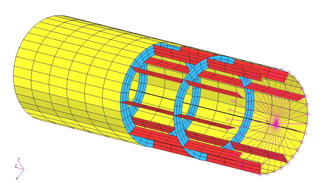 |
Machine Learning, Nonlinear Buckling (Post-Buckling) Optimization of a Reinforced Cylinder with MSC Nastran SOL 400 A reinforced cylinder is fixed at the base and a load is applied laterally at its top. Machine learning is performed to determine the optimal thicknesses of the reinforcements to achieve a minimum eigenvalue of 30 while minimizing the weight. This example features the optimization of nonlinear responses from MSC Nastran SOL 400 and involves nonlinear buckling (post-buckling) analysis. Starting Files: Link Solution BDF Files: Link |
Link | Link |
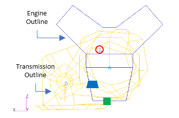 |
Parameter Study, Global Optimization with a Latin Hypercube Design Consider the optimization of a generic engine model that represents a V6 engine and automatic transmission as well as other components such as engine mount, transmission mount, crankshaft, drive axles, and flywheel. The Parameter Study web app is used to configure multiple local optimizations, each with different initial values for the variables, and MSC Nastran is used to perform each optimization. Frequency response plots are created afterward. The process of performing multiple local optimizations, then taking the best, or optimal, design is known as Global Optimization. Starting Files: Link Solution BDF Files: Link |
Link | Link |
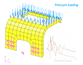 |
Parameter Study, Varying the Location of Concentrated Masses A frequency response analysis is performed on a bracket. The goal in this tutorial is to vary the position of 5 concentrated masses on the bracket and determine the displacement vs. frequency plots for each different configuration of concentrated masses. In total, six MSC Nastran runs are configured, each with a different configuration of the concentrated masses. Starting Files: Link Solution BDF Files: Link |
Link | |
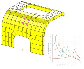 |
Parameter Study, Varying the Position of Extra Supports The location of supports on a structural or mechanical system greatly influences its stiffness. This tutorial discusses one method to vary the location of supports and view displacement vs. frequency plots. Starting Files: Link Solution BDF Files: Link |
Link | |
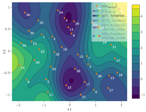 |
Prediction Analysis, Gaussian Process Regression This tutorial demonstrates the use of Gaussian process regression. |
Link | Link |
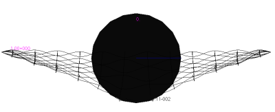 |
Prediction Analysis, Dynamic Impact of a Rigid Sphere on a Woven Fabric Consider a transient analysis of a rigid sphere impacting a woven fabric. The parameters allowed to vary include the friction coefficients. The response of interest are the displacements. This tutorial describes how to configure multiple MSC Nastran runs to generate training data. Gaussian process regression is used to train a surrogate model and make predictions. The prediction performance of the surrogate model is also evaluated. Also discussed are instructions to create displacement vs. time plots. Starting Files: Link Solution BDF Files: Link |
Link | |
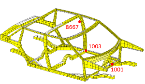 |
Prediction Analysis, Frequency Response Analysis (SOL 111) Consider a frequency response analysis of a ground vehicle. For different configurations of the ground vehicle, there is a desire to rapidly determine the frequency responses, including accelerations and pressures, while keeping the number of Finite Element (FE) solver runs to a minimum. This tutorial describes the procedure to use Gaussian progress regression as a surrogate model for computationally expensive Finite Element (FE) based simulations. This tutorial walks users through the process of acquiring training data, fitting the surrogate model, making predictions and quantifying uncertainty. In addition, the process to screen variables/parameters via Automatic relevance determination (ARD) is discussed. Starting Files: Link Solution BDF Files: Link |
Link | |
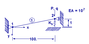 |
Prediction Analysis, Buckling Consider a linear buckling analysis. The parameter allowed to vary is a spring constant. The response of interest is the buckling load factor. This tutorial describes how to configure multiple MSC Nastran runs to generate training data. Gaussian process regression is used to train a surrogate model and make predictions. The prediction performance of the surrogate model is also evaluated. Starting Files: Link Solution BDF Files: Link |
Link | |
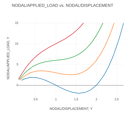 |
Prediction Analysis, Post-Buckling Consider a post-buckling analysis. The parameter allowed to vary is a spring constant. The responses of interest include the applied load and displacements. This tutorial is similar to the previous tutorial named Prediction Analysis, Buckling. Like the previous tutorial, this tutorial discusses the use of Gaussian process (GP) regression to train a surrogate model. To expand your experience with GP regression, this tutorial purposely demonstrates a scenario where a poorly fitted model is obtained and what the procedure is to remedy this issue. Also discussed are instructions to create load vs. displacement plots . Starting Files: Link Solution BDF Files: Link |
Link |
Beams Tutorials
| Title and Description | PDF Tutorial | YouTube Tutorial | |
|---|---|---|---|
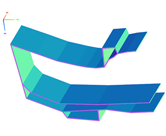 |
Introduction to the PBMSECT Web App This introductory tutorial details the use of the PBMSECT web app to generate arbitrary beam cross sections. The PBMSECT web app is used to automatically generate and manage the following bulk data entries: PBMSECT, PBRSECT, POINT and SET1. |
Link | Link |
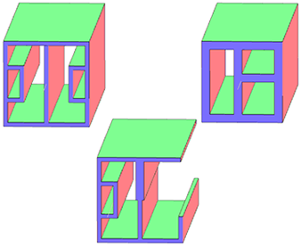 |
Examples of arbitrary beam cross sections with PBMSECT and PBRSECT This tutorial describes the procedure to generate different types of arbitrary beam cross sections, including open or closed profiles. Starting BDF Files: Link Solution BDF Files: Link |
Link | Link |
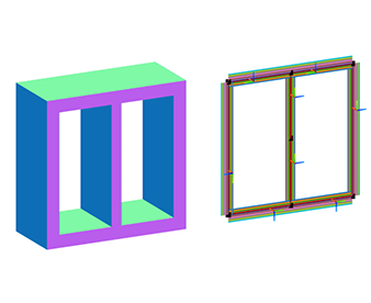 |
Composite Arbitrary Beam Cross Section Composite arbitrary beam cross section (ABCS) may be defined through the use of the PBMSECT and CBEAM3 entries. This tutorial details the use of the PBMSECT web app to construct a composite ABCS and generate the necessary PBMSECT, POINT and SET1 entries. Important considerations, such as ply coordinate systems and validating the FEM of the beam cross section, are discussed. Starting BDF Files: Link Solution BDF Files: Link |
Link | Link |
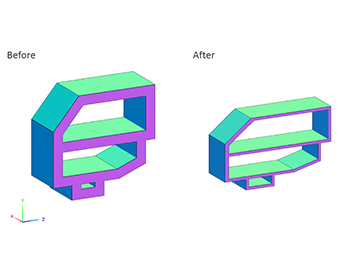 |
Arbitrary Beam Cross Section Optimization MSC Nastran SOL 200 supports varying the width, height and wall thickness of arbitrary beam cross sections (ABCS) defined by the PBRSECT or PBMSECT entries. This tutorial walks you through the process of generating an ABCS via the PBMSECT entry, configuring an optimization for MSC Nastran SOL 200, and reviewing the optimization results. Starting BDF Files: Link Solution BDF Files: Link |
Link | Link |
Composite Laminate Optimization Tutorials
| Title and Description | PDF Tutorial | YouTube Tutorial | |
|---|---|---|---|
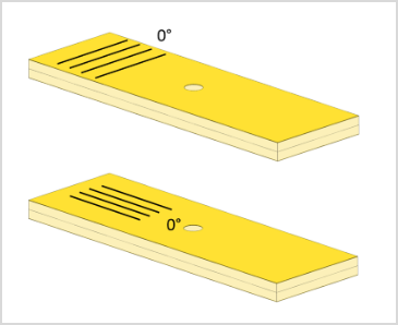 |
Composite Coupon – Phase A – Determination of the optimal 0° direction of a composite The goal of this 5-phase tutorial series is to optimize a composite coupon, with a core, and produce a lightweight composite that satisfies failure index constraints. The optimal ply shapes (ply drop-offs) and ply numbers are determined for 0°, ±45°, and 90° plies. A stacking sequence optimization is performed to satisfy manufacturing requirements. One important part of optimizing composites is visualizing the composite plies. This tutorial series also demonstrates the visualization of ply drop-offs, tapered plies and core layers. This first phase involves determining the optimal 0° direction of a composite. It is best practice to align the 0° plies in the direction of the load. Not doing so will more than likely produce a suboptimal composite that is heavier than necessary. This tutorial demonstrates the use of MSC Nastran's optimizer to determine the optimal 0° direction of a composite. An optimization is performed to maximize the stiffness of the composite for multiple load cases and while varying the angle of the 0° plies. Ultimately, the best 0° direction is determined. This is the first phase in a 5-phase tutorial series. Starting BDF Files: Link Solution BDF Files: Link |
Link | Link |
|
Composite Coupon – Phase B – Baseline Ply Number Optimization This tutorial demonstrates how to configure a basic ply number optimization of continuous plies that span the entire model. The goal of this tutorial is to demonstrate basic actions such as creating variables, a weight objective and constraints on failure index. The results of this ply number optimization serve as a baseline for future comparisons. In a subsequent tutorial, the ply shapes will be optimized to minimize weight. This is the second phase in a 5-phase tutorial series. Starting BDF Files: Link Solution BDF Files: Link |
Link | Link |
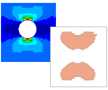 |
Composite Coupon – Phase C – Data Preparation for Ply Shape Optimization This tutorial is a guide to preparing data for ply shape optimization in a subsequent tutorial. The maximum failure index values of the outer plies of the composite are determined and saved to specially formatted PLY000i files. The PLY000i files will be used to construct optimal ply shapes in a subsequent tutorial. This is the third phase in a 5-phase tutorial series. Starting BDF Files: Link Solution BDF Files: Link |
Link | Link |
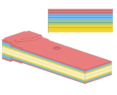 |
Composite Coupon – Phase D – Ply Shape and Ply Number Optimization This tutorial details the process to build optimal ply shapes and perform a ply number optimization. The optimal ply shapes are constructed to follow the contours of the failure indices. The ply number optimization involves minimizing weight and constraining the failure indices of plies. The PLY000i files and BDF files from the previous tutorial, phase C, are used in this tutorial. This is the fourth phase in a 5-phase tutorial series. Starting BDF Files: Link Solution BDF Files: Link |
Link | Link |
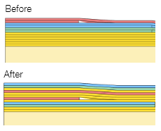 |
Composite Coupon – Phase E – Stacking Sequence Optimization This tutorial involves performing a stacking sequence optimization and is a continuation of the previous tutorial, phase D. A final statics analysis is performed to confirm the optimized composite satisfies failure index constraints. This is the fifth phase in a 5-phase tutorial series. Starting BDF Files: Link Solution BDF Files: Link |
Link | Link |
| Title and Description | PDF Tutorial | YouTube Tutorial | |
|---|---|---|---|
 |
Sandwich Composite Panel – Phase B – Baseline Core Thickness Optimization The goal of this 3-phase tutorial series is to optimize a curved composite panel, with a core, and produce a lightweight composite that satisfies constraints on the buckling load factor. This tutorial series focuses exclusively on optimizing the thickness of the core. The methods detailed in the tutorial series are applicable to both foam and honeycomb cores. This tutorial demonstrates how to configure a basic core thickness optimization where the core has a constant thickness throughout the entire model. The goal of this tutorial is to demonstrate basic actions such as creating variables, a weight objective and constraints on the buckling load factor. The results of this core thickness optimization serve as a baseline for future comparisons. In a subsequent tutorial, the core will be allowed to have a variable thickness throughout the model and will be optimized to minimize weight. This is the first phase in a 3-phase tutorial series. Starting BDF Files: Link Solution BDF Files: Link |
Link | Link |
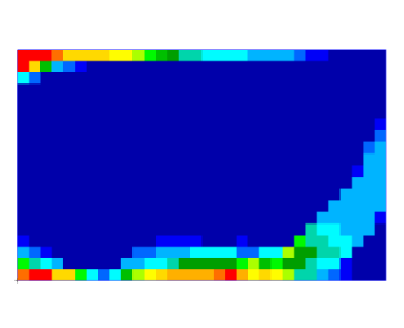 |
Sandwich Composite Panel – Phase C – Topometry Optimization to Determine Optimal Core Shape This tutorial is a guide to preparing data for core shape and core thickness optimization in a subsequent tutorial. A topometry optimization is performed in this tutorial to determine the ideal thickness distribution of the core throughout the entire composite panel while satisfying constraints on the buckling load factor and minimizing weight. The results of a topometry optimization are contained in the PLY000i files and will be used to construct optimal core shapes in a subsequent tutorial. This is the second phase in a 3-phase tutorial series. Starting BDF Files: Link Solution BDF Files: Link |
Link | Link |
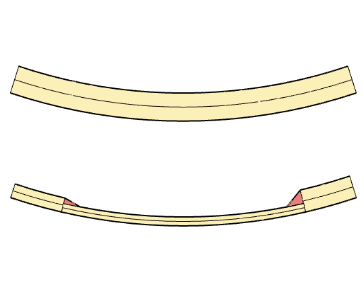 |
Sandwich Composite Panel – Phase D – Core Shape and Core Thickness Optimization This tutorial details the process to build optimal core shapes and perform a core thickness optimization. The optimal core shapes are constructed to follow the contours of thickness results generated by a topometry optimization. The core thickness optimization involves minimizing weight and constraining the buckling load factor. The PLY000i files and BDF files from the previous tutorial, phase C, are used in this tutorial. Comparisons are made between this optimization in phase D and the baseline optimization performed in phase B. This is the third phase in a 3-phase tutorial series. Starting BDF Files: Link Solution BDF Files: Link |
Link | Link |
Shape Optimization Tutorials
| Title and Description | PDF Tutorial | YouTube Tutorial | |
|---|---|---|---|
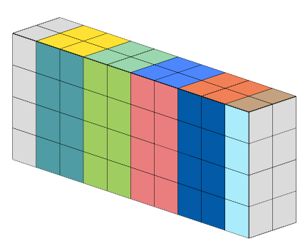 |
Shape Optimization of a Cantilever Beam This tutorial is an introduction to MSC Nastran's Shape Optimization capability. A cantilever beam is configured for a shape optimization. The goal is to minimize the mass while satisfying stress constraints. Specified regions of the beam are allowed to expand or contract and define the shapes that will vary during the optimization. This tutorial discusses the following concepts: auxiliary models, shape basis vectors, scaling shape basis vectors, configuring variable bounds, strategies to prevent mesh distortions, results interpretation, updating the model, and more. Starting BDF Files: Link Solution BDF Files: Link |
Link | Link |
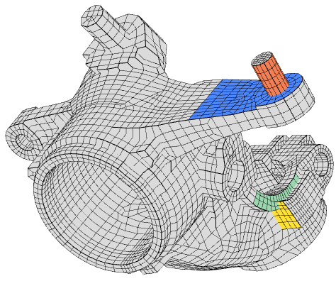 |
Shape Optimization of a Steering Knuckle A steering knuckle is configured for a shape optimization. The goal is to minimize the mass while satisfying stress constraints. Twelve load cases are considered. Four regions of the model are allowed to expand or contract and define the shapes that will vary during the optimization. This tutorial is an advanced shape optimization tutorial and utilizes MSC Nastran's shape optimization capability. Starting BDF Files: Link Solution BDF Files: Link |
Link | Link |
Post-processor Tutorials
| Title and Description | PDF Tutorial | YouTube Tutorial | |
|---|---|---|---|
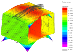 |
MSC Nastran Results - Introduction to Nastran Results - Displacements, forces, stresses and composite ply stresses for entries CQUAD4, CTRIA3, CQUAD8, CBEAM, CBUSH, CFAST, PSHELL, PCOMP, PBMSECT, PBUSH and PFAST
This tutorial is an introduction to Nastran results.
Starting BDF Files: Link |
Link | Link |
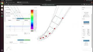 |
MSC Nastran Results - CBAR - Element forces, stresses and displacements
The goal of this exercise is to review the results from a statics analysis. The element forces, bending stresses, displacements and twist of CBAR elements is displayed. Source of Exercise Problem 1: Linear Statics, Rigid Frame Analysis Patran Reference Manual, Part 6: Results Postprocessing, Chapter 15 - Verification and Validation Starting BDF Files: Link |
Link | |
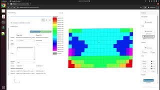 |
MSC Nastran Results - PCOMP - Ply stresses
The goal of this exercise is to view the ply stresses of a 3 layer composite laminate. Source of Exercise Problem 2: Linear Statics, Cross-Ply Composite Plate Analysis Patran Reference Manual, Part 6: Results Postprocessing, Chapter 15 - Verification and Validation Starting BDF Files: Link |
Link | |
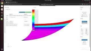 |
MSC Nastran Results - CQUAD4 - Stresses and deformations in spherical coordinates
The goal of this exercise is to inspect the deformation and stresses of an FE model configured in the spherical coordinate system. Source of Exercise Problem 5: Linear Statics, 2D Shells in Spherical Coordinates Patran Reference Manual, Part 6: Results Postprocessing, Chapter 15 - Verification and Validation Starting BDF Files: Link |
Link | |
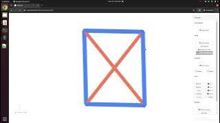 |
MSC Nastran Results - CROD - Axial forces and stresses
The goal of this exercise is to plot the deformations, axial forces and stresses of CROD elements. Source of Exercise Problem 8: Linear Statics, Pinned Truss Analysis Patran Reference Manual, Part 6: Results Postprocessing, Chapter 15 - Verification and Validation Starting BDF Files: Link |
Link | |
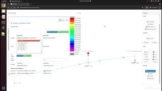 |
MSC Nastran Results - CGAP - Element force and stresses in CGAP elements
The goal of this exercise is to inspect the element forces and displacements in CGAP elements. Source of Exercise Problem 13: Nonlinear Statics, Beams with Gap Elements Patran Reference Manual, Part 6: Results Postprocessing, Chapter 15 - Verification and Validation Starting BDF Files: Link |
Link | |
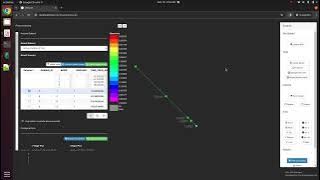 |
MSC Nastran Results - CONM2 and CELAS1 - Natural Frequencies, Mode Shapes, Spring Mass
The goal of this exercise is to inspect the natural frequencies and mode shapes of a spring mass system. Source of Exercise Problem 14: Normal Modes, Point Masses and Linear Springs Patran Reference Manual, Part 6: Results Postprocessing, Chapter 15 - Verification and Validation Starting BDF Files: Link |
Link | |
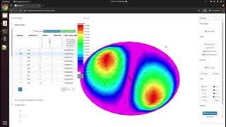 |
MSC Nastran Results - CTRIA - Natural Frequencies, Mode Shapes, Cylindrical Coordinates
The goal of this exercise is to inspect the natural frequencies and mode shapes of an FE model composed of CTRIA elements. Source of Exercise Problem 16: Normal Modes, Pshells and Cylindrical Coordinates Patran Reference Manual, Part 6: Results Postprocessing, Chapter 15 - Verification and Validation Starting BDF Files: Link |
Link | |
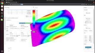 |
MSC Nastran Results - Buckling Load Factor of a Thin Walled Cylinder
The goal of this exercise is to determine the eigenvalue from a buckling analysis and determine the buckling load. Source of Exercise Problem 17: Buckling, shells and Cylindrical Coordinates Patran Reference Manual, Part 6: Results Postprocessing, Chapter 15 - Verification and Validation Starting BDF Files: Link |
Link | |
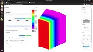 |
MSC Nastran Results - CHEXA - Transient Analysis in Cylindrical Coordinates
The goal of this exercise is to view the displacements of a static and transient analysis. The process to create displacement vs. time plots is also demonstrated. Source of Exercise Problem 19: Direct Transient Response, Solids and Cylindrical Coordinates Patran Reference Manual, Part 6: Results Postprocessing, Chapter 15 - Verification and Validation Starting BDF Files: Link |
Link | |
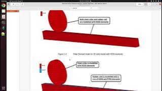 |
MSC Nastran SOL 400 Results - Displacements, forces of a steel roller moving on rubber
The displacements are displayed for a steel roller moving on a rubber base. Special consideration is given to the steel roller. A load vs. displacement plot is created for the steel roller. Source of Exercise Chapter 5: Steel Roller on Rubber MSC Nastran 2023.3 Demonstration Problems Manual - Implicit Nonlinear Starting BDF Files: Link |
Link | |
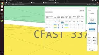 |
MSC Nastran SOL 400 Results - CBUSH,CFAST,CWELD - Shear Forces in Fasteners of a Lap Joint
The shear forces in fasteners of a lap joint are displayed. The fasteners are modeled with CBUSH, CFAST and CWELD elements. Source of Exercise Chapter 33: Large Rotation Analysis of a Riveted Lap Joint MSC Nastran 2023.3 Demonstration Problems Manual - Implicit Nonlinear Starting BDF Files: Link |
Link | |
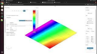 |
MSC Nastran SOL 400 Results - Load vs. Deflection Graph (Load Stroke Plot)
This exercise the procedure to create load vs. deflection graphs, also known as load stroke plots. Source of Exercise Chapter 36: Shallow Cylindrical Shell Snap-through MSC Nastran 2023.3 Demonstration Problems Manual - Implicit Nonlinear Starting BDF Files: Link |
Link |
Uncertainty Quantification
| Title and Description | PDF Tutorial | YouTube Tutorial | |
|---|---|---|---|
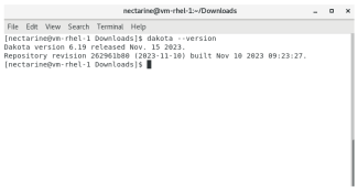 |
Uncertainty Quantification - Installing Sandia Dakota on Windows and Red Hat Linux 7 This tutorial details the process to download and configure Sandia Dakota on Windows and Red Hat Linux 7. |
Link | |
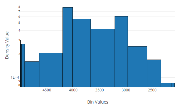 |
Uncertainty Quantification - 10 Bar Truss with MSC Nastran This example details the use of uncertainty quantification to reduce the variability of responses when uncertain parameters are present. Forward propagation of uncertainty is the focus of this exercise and the sampling method is used for uncertainty quantification. A 10 bar truss with 4 uncertain parameters is considered and a Latin Hypercube sampling is used. The quantities of interest include the mean and standard deviation values of the responses and correlation coefficients between the inputs (parameters) and outputs (responses). Starting BDF Files: Link Solution BDF Files: Link |
Link |
Optimization Under Uncertainty
| Title and Description | PDF Tutorial | YouTube Tutorial | |
|---|---|---|---|
|
Optimization Under Uncertainty - 3 Bar Truss, Part 1 of 2 There are many methods available for uncertainty quantification to approximate statistics such as mean, standard deviation and tail probabilities of stochastic responses. Each method has its own computational cost. During an optimization under uncertainty (OUU), an uncertainty quantification (UQ) is performed frequently. If the cost of each UQ is high, the OUU’s computational costs will also be prohibitively high. The mean value first-order second-moment (MVFOSM) method is one of the least expensive UQ methods and involves one black box function evaluation to acquire the response values and gradients. From a single evaluation, the required statistics are approximated, and is a contrast to other UQ methods that may require dozens or hundreds of black box function runs. The MVFOSM is limited to responses that are linear and normally (Gaussian) distributed and is not universally appropriate. This exercise details a procedure to determine if the MVFOSM method is appropriate to approximate the statistics of stress responses of a 3-bar truss. If the MVFOSM is suitable, this will significantly reduce the number of black box function runs necessary to perform the UQ and OUU. The black box function is the FEA solver MSC Nastran. MSC Nastran is used to perform the finite element analysis and acquire responses and gradients. Sandia Dakota is used to perform the UQ. The SOL 200 Web App is used to configure the UQ. This is part 1 of a 2-part tutorial. Starting BDF Files: Link Solution BDF Files: Link |
Link | Link |
|
Optimization Under Uncertainty - 3 Bar Truss, Part 2 of 2 This example details the process to configure and perform an optimization under uncertainty (OUU) for a 3-bar truss. Also, details are included regarding how to interpret the OUU results and final probabilities of failure. The uncertainty quantification (UQ) is performed via the mean value first-order second-moment (MVFOSM) method. This is part 2 of a 2-part tutorial. The optimization problem statement is to minimize the mean mass while ensuring the stress constraints have a probability of failure no greater than 5%. MSC Nastran is used to perform the finite element analysis and acquire responses and gradients. Sandia Dakota is used to perform the UQ and OUU. The SOL 200 Web App is used to configure the OUU and will automatically exchange responses and gradients between MSC Nastran and Sandia Dakota. Starting BDF Files: Link Solution BDF Files: Link |
Link | Link |
 |
Optimization Under Uncertainty - 53 Bar Truss Both uncertainty quantification (UQ) and optimization under uncertainty (OUU) may require hundreds or thousands of black box function evaluations when considering a large number of uncertain variables. Certain black box functions will require hours or days for a single run, so thousands of black box function evaluations are impractical. Finite element solvers are such black box functions where at most a few hundred runs are practical. This tutorial details how to configure an OUU when a large number of uncertain variables are considered, and strategies are discussed to minimize the number of black box function runs. The OUU involves minimizing the mass of a 53-bar truss, varying the mean cross section area of 53 truss members (53 variables), and constraining the probability of failure to 5%, where failure occurs if the axial stress exceeds the material yield strength. This OUU may require 200 to 2000 black box function runs, so the strategies discussed are critical to reduce the number of runs necessary to converge to a solution. The black box function is the FEA solver MSC Nastran. MSC Nastran is used to perform the finite element analysis and acquire responses and gradients. Sandia Dakota is used to perform the UQ and OUU. The SOL 200 Web App is used to configure the OUU. Starting BDF Files: Link Solution BDF Files: Link |
Link | Link |
|
Robust Design Optimization - Acoustic Box Small deviations to structural or mechanical systems during manufacturing can result in significantly varying performance. Examples of varying performance include variations in hole diameters that can lead to variations in peak stress, and variations in gauge thicknesses that can lead to variations in acoustic peak pressures. This tutorial details the use of robust design optimization to reduce the variability of performance when input uncertainties are considered. Specifically, a robust design optimization is configured and performed to minimize the variability of responses. A finite element model is considered of an acoustic box subjected to a dynamic load. The uncertain variables correspond to the gauge thicknesses of the acoustic box. The robust design objective is to minimize the sum of mean and 3-standard deviations of peak acoustic pressures at 2 locations of the FE model. A constraint on mean mass is imposed. The FE solver MSC Nastran is used to perform the acoustic analysis and acquire the necessary responses. Sandia Dakota is used to perform the uncertainty quantification and robust design optimization. The SOL 200 Web App is used to configure both the uncertainty quantification and robust design optimization. Starting BDF Files: Link Solution BDF Files: Link |
Link | Link |
Guidance on Configuring a Single Scalar Objective
Failure to do this will result in a USER FATAL MESSAGE similar to the one below.
 *** USER FATAL MESSAGE 7147 (DPR3H1)
     THE DESOBJ COMMAND WITH ID =  9000000 REFERENCES A DRESP2   ENTRY WHICH IN
     TURN REFERENCES DRESP1 ID =  8000003 WHICH INVOKES MULTIPLE RESPONSES.
     USER INFORMATION: THE DRESP1 ENTRIES INVOLVED IN DEFINING THE OBJECTIVE MUST BE SCALAR QUANTITIES.
     USER ACTION     : IF YOUR DRESP2 REFERENCES A DRESP1 THAT DEFINES A RESPONSE LIKE MAX OR RSS,
     MAKE SURE TO USE FLAG 'DRESP2' INSTEAD OF 'DRESP1' ON THE CONTINUATION LINE.
Examples of Acceptable and Unacceptable Objectives
A standard objective is configured with the PTYPE, ATTA, ATTB and ATTi fields. Different configurations of these fields can produce single or multiple responses. Only an objective that yields a single scalar response is acceptable.| Configuration | Explanation |
|---|---|
|
Objective, r0
Let r0 be defined as shown below. The label r0 is described as "The x displacement of GRID 1." 
|
Since r0 is associated with 1 value (1 components x 1 GRID), the DRESP1 entry
yields 1 value.
This is an acceptable objective. |
|
Objective, r0
Let r0 be defined as shown below. The label r0 is described as "The x and y displacements of GRIDs 1, 2 and 3." 
|
Since r0 is associated with 6 values (2 components x 3 GRIDs), the DRESP1 entry
yields 6 values.
This is an unacceptable objective. |
|
Objective, r0
Let r0 be defined as shown below. The label r0 is described as "The z frequency displacement for all forcing frequencies at GRID 1101." 
|
Assume there are 100 forcing frequencies. The label r0 will yield 100 z-displacement
values for GRID 1101.
This is an unacceptable objective. |
|
Objective, S0
Let S0 be defined as shown below. The label S0 is described as "Take the AVG or average z frequency displacements for all forcing frequencies at GRID 1101." 
|
Since the ATTB is set to AVG or average, S0 will be the average displacement across
the forcing frequency range. The label S0 ultimately yields one value.
This is an acceptable objective. |
Examples of Acceptable and Unacceptable Equation Objectives
Generally, to achieve an acceptable equation objective each argument/label of the equation must be associated with only a single scalar response.| Configuration | Explanation |
|---|---|
|
Equation Objective, R0: g(a1) = a1
a1: Let a1 be defined as shown below. The label a1 is described as "The vonMisses stress of element 1." 
|
Since a1 is associated with only one value, the equation R0 evaluates to one value.
This is an acceptable objective equation. |
|
Equation Objective, R0: g(a1) = a1
a1: Let a1 be defined as shown below. The label a1 is described as "The vonMisses stress of any element associated with PSHELL 101." 
|
Suppose PSHELL 101 is associated with 100 elements. The label a1 is associated with
100 values (1 stress value x 100 elements). Ultimately, the equation R0
evaluates to 100 values.
This is an unacceptable objective equation. |
Response Types and Ideal Configurations for a Single Scalar Response
| Response Type | Configuration to Yield a Single Scalar Response |
|---|---|
|
These responses always generate a single value and can be used as an objective. |
|
|
|
|
|
|
|
|
|
|
|
|
|
|
Frequently Asked Questions
-
Q: Can the design variable labels be customized?
A: A limited level of label customization is supported. All labels are strictly in the form: qi. For example, x101 and r3400.- q - The letter q is dependent on the section, e.g. x for design variables, y for custom design variables, r for constraints, etc.
- i - This is a positive integer. The labels can only be changed via the CSV Export/Import capability and must honor the strict form of qi, e.g. a label such as x1 can be changed to x101, but a label such as y1 cannot be changed to T_PANEL1.
-
Q: For user supplied IDs such as GRID IDs, ELEM IDs and PIDs,
does the web app check to make sure the ID exists?
A: Only PIDs are checked. When specifying the ATTi input for responses or constraints, the web app only checks if the IDs exist for MSC Nastran property entries, e.g. PSHELL, PCOMP, etc. All other IDs are not checked, e.g. GRID IDs, ELEM IDs, etc.
Uploading BDF Files
Uploading files to the web app is best described in one sentence:
Every file MSC Nastran needs to run should also be uploaded to the web app.
Consider an example model that consists of the following file set:
car_model.bdf (Currently not set to SOL 200)
door_left.bdf
door_right.bdf
hood.dat
frame.bdf
When running an analysis with MSC Nastran, only one file, car_model.bdf, must be specified and MSC Nastran, upon execution, will search for the other files. For this example, MSC Nastran needs 5 files to run.
When uploading BDF files to the web app, EACH file must be manually selected.
As shown in the image below, 5 files have been manually selected and uploaded.
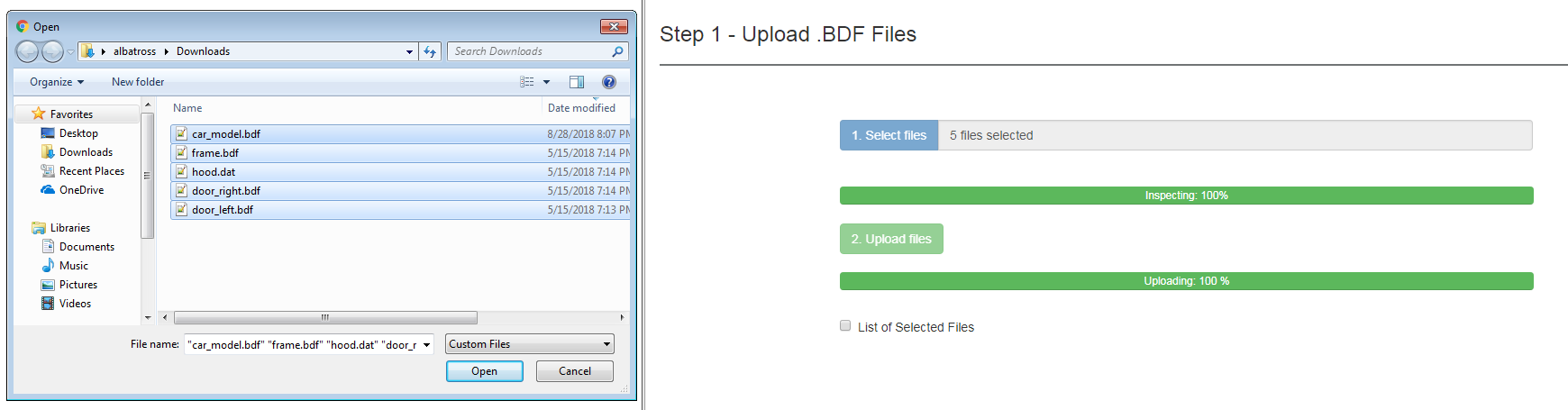 Downloading Files
Generally, upon download from the web app, two BDF files will be downloaded from the web app.
model.bdf (Formerly car_model.bdf, but has been set for SOL 200)
design_model.bdf (Contains entries for the design model)
These files must be combined with the original file set. The optimization is then performed by providing one file, model.bdf, to MSC Nastran. For this example, this is the new file set:
model.bdf (Formerly car_model.bdf)
design_model.bdf
door_left.bdf
door_right.bdf
hood.dat
frame.bdf
Re-Uploading SOL 200 Files
A previous design model downloaded from the SOL 200 Web App can be re-uploaded in the future. Upon re-upload, changes to the design model, such as design variable, objective or constraint changes may be performed.
Like before each file MSC Nastran needs to run should also be provided to the web app.
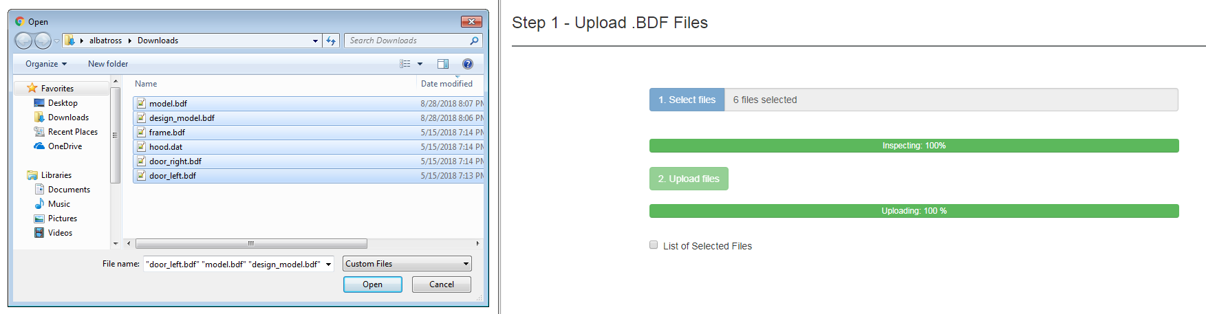
One exception to this procedure is the Multi Model Optimization web app. For each design model uploaded to the app, only the following and respective files are needed: model.bdf and design_model.bdf.
Downloading Files and Executing MSC Nastran
There are two options for downloading .bdf files from the SOL 200 Web App. Both options are summarized below. Option 1 is the preferred method.
Option 1 - Auto Execute MSC Nastran
This option will download the following files:
- nastran_working_directory.zip
- This option will download a new file named "nastran_working_directory.zip"
- Right click on the new .zip file and select "Extract All." A new folder is created.
- Within this new folder is a shortcut named Start MSC Nastran. Double click this shortcut.
- If there are any additional windows, click Open, Run or Allow Access in each window.
- MSC Nastran will now be executed and after MSC Nastran is finished, results will be automatically uploaded to the SOL 200 Web App.
This option will perform 3 actions:
- MSC Nastran will be automatically started. This step will be skipped if there is an existing .f06 file in the folder.
- A Status page will be opened and tracks the progress of MSC Nastran.
- If MSC Nastran finishes successfully, a Results page will be opened. If there is a FATAL MESSAGE in the .f06, the Results page will not be opened.
This executable has been tested ONLY on Windows 10 and Red Hat Linux 7.x. In order for this executable to work successfully, the following conditions must be met. Failure to meet any of these requirements will cause the executable to terminate early before starting MSC Nastran.
- MSC Nastran is installed in the default location (Windows - C:\MSC.Software\MSC_Nastran, Linux - /msc/MSC_Nastran) OR the PATH environment variable has been configured with the installation location.
- Any INCLUDE files must be in the same directory.
- The machine running MSC Nastran must have network access to the SOL 200 Web App.
- A compatible must be installed in the default location.
If performing any of the following, the MSC Nastran utility MultiOpt is to be used:
- Global Optimization
- Global Optimization Type 2
- Parameter Study
- Multi Model Optimization
If using MultiOpt,
- the MSC_LICENSE_FILE environment variable is configured with the location to the license.
- the folder name does not contain any spaces or special characters such as ( ! @ # $ %.
Option 2 - Download BDF Files
This option will download the following files:
- model.bdf
- design_model.bdf
- GO.xml or MMO.xml
If performing Local Optimization or Sensitivity Analysis
- Find and double click the MSC Nastran desktop shortcut.
- Select the model.bdf file.
- Click Run.
If performing any of the following, the MSC Nastran utility MultiOpt is to be used:
- Global Optimization
- Global Optimization Type 2
- Parameter Study
- Multi Model Optimization
If using MultiOpt, do the following:
- Open the command prompt.
- Navigate to the folder containing the model.bdf, design_model, GO.xml or MMO.xml files.
cd Downloads\nastran_working_directory
- Use this command to start MSC Nastran (If MMO.xml is present, use MMO.xml instead of GO.xml)
msc20180 MultiOpt GO.xml
. - The msc20180 word will depend on the version of MSC Nastran being used. This will only work
if:
- The PATH environment variable is properly configured with the location of the MSC Nastran installation.
- The MSC_LICENSE_FILE environment variable has been configured.
Optimization Types
| Type | Results File | Description |
|---|---|---|
| Local Optimization | .f06 | A regular optimization is performed. |
| Sensitivity Analysis | .csv | A sensitivity analysis is performed only for the INITIAL design. |
| Global Optimization | multiopt.log | The native Global Optimization capability in MSC Nastran's is used. The final results are contained in the multiopt.log file. |
| Global Optimization Type 2 | Multiple .f06 files |
This is a non-native Global Optimization method. A portion of this procedure is
performed by MSC Nastran, while the rest of the procedure is performed by
an executable available in Option 1 - Auto Execute MSC Nastran.
Overview of Procedure
|
| Parameter Study | Multiple .f06 files |
This is a non-native method. A portion of this procedure is
performed by MSC Nastran, while the rest of the procedure is performed by
an executable available in Option 1 - Auto Execute MSC Nastran.
Overview of Procedure
|
Supported Capabilities
A majority of MSC Nastran's SOL 200 capabilities are supported by the SOL 200 Web App. This section discusses which specific capabilities are supported.
Capabilities
- Optimization Types
- Size
- Topometry
- Topology
- Topography
- Optimization Options
- Local Optimization
- Sensitivity Analysis
- Global Optimization
- Parameter Study
- Multi Model Optimization
- Machine Learning
- Analysis Types
- SOL 101 - Statics
- SOL 103 - Normal Modes
- SOL 105 - Buckling
- SOL 107 - Direct Complex Eigenvalues
- SOL 108 - Direct Frequency Response
- SOL 110 - Modal Complex Eigenvalues
- SOL 111 - Modal Frequency Response
- SOL 112 - Modal Transient Response
- SOL 144 - Static Aeroelastic Response
- SOL 145 - Aerodynamic Flutter
- SOL 400 - Implicit Nonlinear (Machine Learning only)
- Multidisciplinary Optimization
- Specify different ANALYSIS types per SUBCASE
- INCLUDE file support
- Equation driven objective and constraints (DRESP2 and DEQATN)
- Objective and constraints dependent on multiple load cases or SUBCASEs (DRSPAN)
- CSV Import/Export - Generate hundreds of Variables, DLINK entries and Constraints
- Semi-automatic Nastran execution and live status updates
- Auto Plotting of Results - Line plots and bar charts
- Model Matching
Supported MSC Nastran Entries
The following lists the MSC Nastran entries supported by the web app. For example, if using the Size web app, DESVAR, DVPREL1, ... entries are generated.
| Bulk Data Entries | |||
|---|---|---|---|
| BEADVAR | x | ||
| DCONADD | x | ||
| DCONSTR | x | ||
| DDVAL | x | ||
| DEQATN | x | ||
| DESVAR | x | ||
| DLINK | x | ||
| DOPTPRM | x | ||
| DRESP1 | x | ||
| DRESP2 | x | ||
| DTABLE | x | ||
| DVXREL1 | x | ||
| DVXREL2 | x | ||
| TOMVAR | x | ||
| TOPVAR | x | ||
| Case Control Commands | |||
| ANALYSIS | x | ||
| DESGLB | x | ||
| DESSUB | x | ||
| DRSPAN | x | ||
| DSAPRT | x | ||
Supported Designable Parameters
| Entry | Designable Parameters |
|---|---|
| Properties | |
| PACABS | CUTFR, B, K, M |
| PACBAR | MBACK, MSEPTM, FRESON, KRESON |
| PBAR | A, I1, I2, J, NSM, C1, C2, D1, D2, E1, D2, F1, F2, K1, K2, I12 |
| PBARL | DIMi, NSM |
| PBEAM | (A(i), I1(i), I2(i), I12(i), J(i), NSM(i), C1(i), C2(i), D1(I), D2(i), E1(i), E2(i), F1(i), F2(i), i = A, B, 1 ... 9), K1, K2, S1, S2, (NSI(j), CW(j), M1(j), M2(j), N1(j), N2(j), j = A, B) |
| PBEAML | (DIMi(j), NSM(j), j = A, B, 1 ... 9) |
| PBRSECT / PBMSECT | W (Overall Width), H(Overall Height),T(Overall Thickness) and T(n) Thickness of segment. |
| PBUSH | (Ki, Bi, GEi, i = 1, 6), SA, ST, EA, ET |
| PBUSH1D | K, C, M, SA, SE |
| PCOMP | Z0, NSM, SB, TREF, GE, Ti, THETAi |
| PDAMP | B1, B2, B3, B4 |
| PELAS | K1, GE1, S1, K2, GE2, S2 |
| PGAP | U0, F0, KA, KB, KT, MU1, MU2 |
| PCOMPG | Z0, NSM, SB, TREF, GE, |
| PMASS | M1, M2, M3, M4 |
| PROD | A, J, C, NSM |
| PSHEAR | T, NSM, F1, F2 |
| PSHELL | T, 12I/T**3, TS/T, NSM, Z1, Z2 |
| PTUBE | OD, T, NSM |
| PVISC | CE1, CR1, CE2, CR2 |
| GPLY | T, THETA |
| PWELD* | D |
| PFAST* | D, KT1, KT2, KT3, KR1, KR2, KR3, MASS, GE |
| Material Properties | |
| MAT1 | E, G, NU, RHO, A, TREF, GE |
| MAT2 | G11, G12, G13, G22, G23, G33, RHO, A1, A2, A3, TREF, GE |
| MAT3 | EX, ETH, EZ, NUXTH, NUZTH, NUZX, RHO, GZX, AX, ATH, AZ, TREF, GE |
| MAT8 | E1, E2, NU12, G12, G1Z, G2Z, RHO, A1, A2, TREF, Xt, Xc, Yt, Yc, S, GE |
| MAT9 | G11, G12, G13, G14, G15, G16, G22, G23, G24, G25, G26, G33, G34, G35, G36, G44, G45, G46, G55, G56, G66, RHO, A1, A2, A3, A4, A5, A6, TREF, GE |
| MAT10 | BULK, RHO, C, GE |
| Connectivity Properties | |
| CBAR | X1, X2, X3, W1A, W2A, W3A, W1B, W2B, W3B |
| CBEAM | X1, X2, X3, BIT, W1A, W2A, W3A, W1B, W2B, W3B |
| CBUSH | X1, X2, X3, S, S1, S2, S3 |
| CDAMP2,4 | B |
| CELAS2 | K, GE, S |
| CELAS4 | K |
| CGAP | X1, X2, X3 |
| CMASS2,4 | M |
| CONM1 | M11, M21, M22, M31, M32, M33, M41, M42, M43, M44, M51, M52, M53, M54, M55, M61, M62, M63, M64, M65, M66 |
| CONM2 | M, X1, X2, X3, I11, I21, I22, I31, I32, I33 |
| CONROD | A, J, C, NSM |
* Not documented in Table 2-1 of the MSC Nastran Design Sensitivity and Optimization User’s Guide but is supported by the DVPREL1 entry
Supported Responses for Objective and Constraints
| DRESP1 | Response Title |
|---|---|
| WEIGHT | Weight |
| VOLUME | Volume |
| EIGN | Eigenvalue |
| CEIG | Complex Eigenvalue |
| FREQ | Frequency |
| LAMA | Buckling Eigenvalue/Factor |
| DISP | Displacement |
| STRAIN | Strain |
| ESE | Element Strain Energy |
| STRESS | Stress |
| FORCE | Force |
| FATIGUE | Fatigue, pseudo-static fatigue analysis |
| FRFTG | Fatigue, random vibration fatigue analysis |
| SPCFORCE | Single Point Constraint Force |
| CSTRAIN | Strain in PCOMP or PCOMPG |
| CSTRESS | Stress in PCOMP or PCOMPG |
| CFAILURE | Composite Failure Criterion |
| CSTRAT | Composite Strength Ratio |
| TOTSE | Total Strain Energy |
| GPFORCE | Grid Point Force |
| GPFORCP | Grid Point Force, PARAM NEOLOP > 1 |
| ABSTRESS | Beam Stresses referencing PBRSECT and PBMSECT |
| FRDISP | Displacement |
| PRES | Acoustic Pressure |
| FRVELO | Velocity |
| FRACCL | Acceleration |
| FRSPCF | Single Point Constraint Force |
| FRSTRE | Element Stress |
| FRFORC | Element Force |
| PSDDISP | Power Spectral Density Displacement |
| PSDVELO | Power Spectral Density Velocity |
| PSDACCL | Power Spectral Density Acceleration |
| RMSDISP | Root Mean Square Displacement |
| RMSVELO | Root Mean Square Velocity |
| RMSACCL | Root Mean Square Acceleration |
| ACPWR | Acoustic Power through Radiated Surface, Panels |
| ACINTS | Acoustic Intensity Normal to Wetted Surface |
| AFPRES | Acoustic Pressure for Acoustic Field Point Mesh (AFPM) |
| AFINTS | Acoustic Intensity for Acoustic Field Point Mesh (AFPM) |
| AFVELO | Particle Velocities for Acoustic Field Point Mesh (AFPM) |
| AFPWR | Acoustic Power for Acoustic Field Point Mesh (AFPM) |
| ERP | Equivalent Radiated Power (ERP) |
| TDISP | Displacement |
| TVELO | Velocity |
| TACCL | Acceleration |
| TSPCF | Single Point Constraint Force |
| TSTRE | Element Stress |
| TFORC | Element Force |
| STMONP1 | Structural Integrated Load Monitor Point |
| STMOND1 | Structural Displacement Monitor Point |
| MONPNT3 | Integrated Load Monitor Point |
| AEMONP1 | Aerodynamic Integrated Load Monitor Point |
| AEMOND1 | Aerodynamic Displacement Monitor Point |
| TRIM | Trim Variable |
| STABDER | Stability Derivative |
| FLUTTER | Flutter Damping Value |
| DIVERG | Dynamic Response of the Selected Root |
| WMPID | Weight from Particular Material or Property ID |
| COMP | Compliance (Product of displacement and the applied load) |
| FRMASS | Fractional Mass |
Supported Bulk Data Entries and Fields
The following depicts bulk data entries and their specific fields that are supported by the web app.
| Field not supported |
| Bulk Data Entry | 2 | 3 | 4 | 5 | 6 | 7 | 8 | 9 |
|---|---|---|---|---|---|---|---|---|
| BEADVAR | ID | PTYPE | PID | MW | MH | ANG | BF | SKIP |
| DESVAR | NORM/XD | YD | ZD | CID | XLB | XUB | DELXV* | |
| GRID | NGSET | DGSET | ||||||
| DCONADD | DCID | DC1 | DC2 | DC3 | -etc.- | |||
| DCONSTR | DCID | RID | LALLOW /LID | UALLOW /UID | LOWFQ | HIGHFQ | ||
| DDVAL | ID | DDVAL 1 | DDVAL 2 | DDVAL 3 | DDVAL4 | DDVAL 5 | DDVAL 6 | DDVAL 7 |
| DDVAL 8 | -etc.- | |||||||
| DEQATN | EQID | EQUATION** | ||||||
| EQUATION** (CONT.) | ||||||||
| DESVAR | ID | LABEL | XINIT | XLB | XUB | DELXV* | DDVAL | |
| DLINK | ID | DDVID | C0 | CMULT | IDV1 | C1 | IDV2 | C2 |
| IDV3 | C3 | -etc.- | ||||||
| DRESP1 | ID | LABEL | RTYPE | PTYPE | REGION | ATTA | ATTB | ATT1 |
| ATT2 | -etc.- | |||||||
| DRESP2 | ID | LABEL | EQID or FUNC | REGION | METHOD | C1 | C2 | C3 |
| "DESVAR" | DVID1 | DVID2 | DVID3 | DVID4 | DVID5 | DVID6 | DVID7 | |
| DVID8 | -etc.- | |||||||
| "DTABLE" | LABL1 | LABL2 | LABL3 | LABL4 | LABL5 | LABL6 | LABL7 | |
| LABL8 | -etc.- | |||||||
| "DRESP1" | NR1 | NR2 | NR3 | NR4 | NR5 | NR6 | NR7 | |
| NR8 | -etc.- | |||||||
| "DNODE" | G1 | C1 | G2 | C2 | G3 | C3 | ||
| G4 | C4 | -etc.- | ||||||
| "DVPREL1" | DPIP1 | DPIP2 | DPIP3 | DPIP4 | DPIP5 | DPIP6 | DPIP7 | |
| DPIP8 | DPIP9 | -etc.- | ||||||
| "DVCREL1" | DCIC1 | DCIC2 | DCIC3 | DCIC4 | DCIC5 | DCIC6 | DCIC7 | |
| DCIC8 | DCIC9 | -etc.- | ||||||
| "DVMREL1" | DMIM1 | DMIM2 | DMIM3 | DMIM4 | DMIM5 | DMIM6 | DMIM7 | |
| DMIM8 | DMIM9 | -etc.- | ||||||
| "DVPREL2" | DPI2P1 | DPI2P2 | DPI2P3 | DPI2P4 | DPI2P5 | DPI2P6 | DPI2P7 | |
| DPI2P8 | DPI2P9 | -etc.- | ||||||
| "DVCREL1" | DCI2C1 | DCI2C2 | DCI2C3 | DCI2C4 | DCI2C5 | DCI2C6 | DCI2C7 | |
| DCI2C8 | DCI2C9 | -etc.- | ||||||
| "DVMREL1" | DMI2M1 | DMI2M2 | DMI2M3 | DMI2M4 | DMI2M5 | DMI2M6 | DMI2M7 | |
| DMI2M8 | DMI2M9 | -etc.- | ||||||
| "DRESP2" | NRR1 | NRR2 | NRR3 | NRR4 | NRR5 | NRR6 | NRR7 | |
| NRR8 | -etc.- | |||||||
| "DVLREL1" | DLIL1 | DLIL2 | DLIL3 | DLIL4 | DLIL5 | DLIL6 | DLIL7 | |
| DLIL8 | -etc.- | |||||||
| DTABLE | LABL1 | VALU1 | LABL2 | VALU2 | LABL3 | VALU3 | LABL4 | VALU4 |
| LABL5 | VALU5 | -etc.- | ||||||
| DVCREL1 | ID | TYPE | EID | CPNAME | CPMIN* | CPMAX* | C0 | |
| DVID1 | COEFF1 | DVID2 | COEF2 | DVID3 | COEF3 | -etc.- | ||
| DVMREL1 | ID | TYPE | MID | MPNAME | MPMIN* | MPMAX* | C0 | |
| DVID1 | COEFF1/'PVAL' | DVID2 | COEF2 | DVID3 | COEF3 | -etc.- | ||
| DVPREL1 | ID | TYPE | PID | PNAME/FID | PMIN* | PMAX* | C0 | |
| DVID1 | COEFF1/'PVAL' | DVID2 | COEF2 | DVID3 | COEF3 | -etc.- | ||
| DVCREL2 | ID | TYPE | EID | CPNAME | CPMIN | CPMAX | EQID | |
| "DESVAR" | DVID1 | DVID2 | -etc.- | |||||
| "DTABLE" | LABL1 | LABL2 | -etc.- | |||||
| DVMREL2 | ID | TYPE | EID | MPNAME | MPMIN | MPMAX | EQID | |
| "DESVAR" | DVID1 | DVID2 | -etc.- | |||||
| "DTABLE" | LABL1 | LABL2 | -etc.- | |||||
| DVPREL2 | ID | TYPE | PID | FNAME | PMIN | PMAX | EQID | |
| "DESVAR" | DVID1 | DVID2 | -etc.- | |||||
| "DTABLE" | LABL1 | LABL2 | -etc.- | |||||
| TOMVAR | ID | TYPE | PID | PNAME/FID | XINIT | XLB | XUB | DELXV* |
| DLINK | TID | C0 | C1 | |||||
| DDVAL | DSVID | |||||||
| TOPVAR | ID | LABEL | PTYPE | XINIT* | XLB* | DELXV* | POWER* | PID |
| SYM | CID | MS1 | MS2 | MS3 | CS | NCS | ||
| CAST | CID | DD | DIE | ALIGN | ||||
| EXT | CID | ED | ALIGN | |||||
| TDMIN | TMIN | TVMAX | ||||||
| STRESS | STLIM | |||||||
* The field is imported and exported but is not configurable within the web app. A text editor is recommended to edit the indicated field.
** The special DEQATN functions, e.g. AVG, SUM, ..., are supported.
Installation
Installation Configurations
The "Installation Procedure" section details the installation instructions for the Node JS web server and the SOL 200 Web App on Windows and Linux platforms.
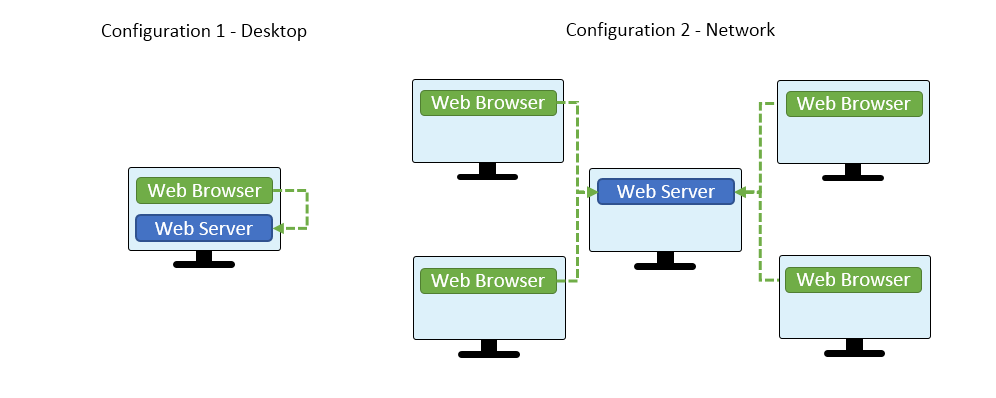
Web Browser Requirements
At least one of the web browsers listed below should be installed to access the SOL 200 Web App.
| Supported Versions | ||
|---|---|---|
| Web Browser | Windows 10 | Linux (RHEL 7.x) |
| Google Chrome | 2021 - Present (v88.0.4324.104 - Present) | 2021 - Present (v88.0.4324.96 - Present) |
| Mozilla Firefox | 2021 - Present (v85.0 - Present) | 2021 - Present (v78.6.1 - Present) |
| Microsoft Edge* | 2021 - Present (v88.0.705.56 - Present) | Browser not available on this platform |
* Microsoft Edge Legacy
 is not supported. Use the new Microsoft Edge
 . Refer to your company’s IT support team for assistance.
Web Server Requirements
Node JS is a free open-source application that will run a web server and host the SOL 200 Web App to other machines.
| Supported Versions | ||
|---|---|---|
| Application | Windows 10 | Linux (RHEL 7.x) |
| Node JS | 2021 - Present (v14.15.4 - Present) | 2021 - Present (v14.15.4 - Present) |
Installation Procedure - Windows
Video Instructions
Instructions
Prerequisites
- Ensure Google Chrome, Mozilla Firefox or Microsoft Edge is installed.
The commands listed in this section are to be executed in the Command Prompt.
- Download the web app ZIP file, e.g. sol_200_web_app.zip
- Extract the contents of the zip file to a folder named: sol_200_web_app
- Licensing - To configure the licensing, following these instructions.
Method A - License File Prerequisites
You have been provided a license file, for example1100101101.dat.
Instructions- A.1 Ensure the license file name includes only the numbers 1 or 0 and the file extension '.dat' (Correct:
1100101101.datIncorrect:for_chris_1100101101.dat) - A.2 Take the license file (example: 10111010.dat) and put it in this directory
./sol_200_web_app/license
- A.1 Ensure the license file name includes only the numbers 1 or 0 and the file extension '.dat' (Correct:
- Download and install the latest version of Node JS
- Windows Installer (.msi), 64-bit: https://nodejs.org/dist/v18.20.5/node-v18.20.5-x64.msi
-
Open the windows command prompt.
If the location of the web app is in restricted directory such asC:\Program Files\sol_200_web_app, the command prompt should be opened with the option "Run as administrator."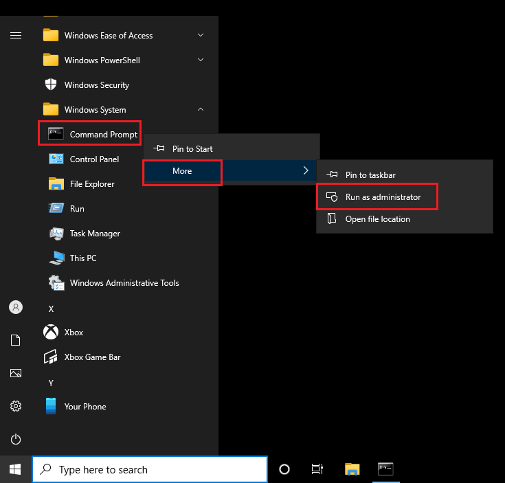
-
Navigate to the directory that contains this file: app.min.js .
cd sol_200_web_app
-
Confirm Node JS has been installed by verifying a version number is available. If a version number is shown, this confirms Node JS has been installed successfully.
node --version
The output of this command will be similar to below but will vary depending on your Node JS version.v16.13.0
If the output is similar to below, the Microsoft HPC Pack is installed on the desktop. This Node application is not the correct version to use. A workaround is provided below.Node Commands Syntax: node {operator} [options] [arguments] Parameters: /? or /help - Display this help message. [...] resume - Resume node [deprecated] For more information about HPC command-line tools, see http://go.microsoft.com/fwlink/?LinkId=120724.As a workaround, try acquiring the Node JS version by using the full path of the Node JS executable."C:\Program Files\nodejs\node.exe" --version v16.13.0
-
To start the web app, type this and run. The first start will ask you to accept the end user license agreement (EULA).
node app.min.js
Important! If the command above does not work, this command may also be used."C:\Program Files\nodejs\node.exe" app.min.js
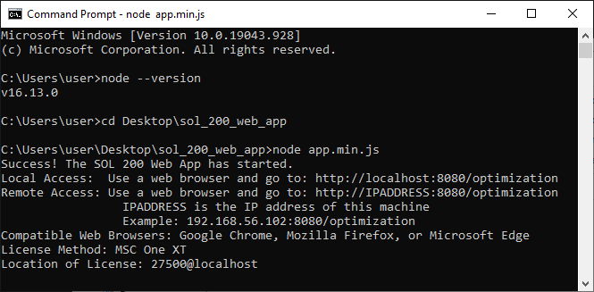
- The Windows Firewall will prompt to select an access option.
- 1) Mark the checkbox for "Public networks, such as those in airports and coffee shops."
- 2) Click "Allow Access." This will open port 8080 on your machine. If this window did not pop up, port 8080 will have to be opened manually using these instructions: Open and Verify Port 8080 of the Server is Open.
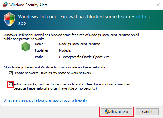
- Open Google Chrome, Mozilla Firefox or Microsoft Edge and go to
localhost:8080/optimization - If you can access the web app, the web app has been successfully installed
- Other machines on the local network can also access the web app. Determine the IP address of the machine that has the web app installed. Use the IP address to access the web app.
For this example, the IP address192.168.56.1has the web app running. Open a web browser and go to this URL to access the web app:192.168.56.1:8080/optimization
If other machines cannot access the web app, it is likely that the IP address is not accessible or the firewall is not configured properly to open port 8080. See this section for additional instructions Enabling Web App Access to Other Devices.
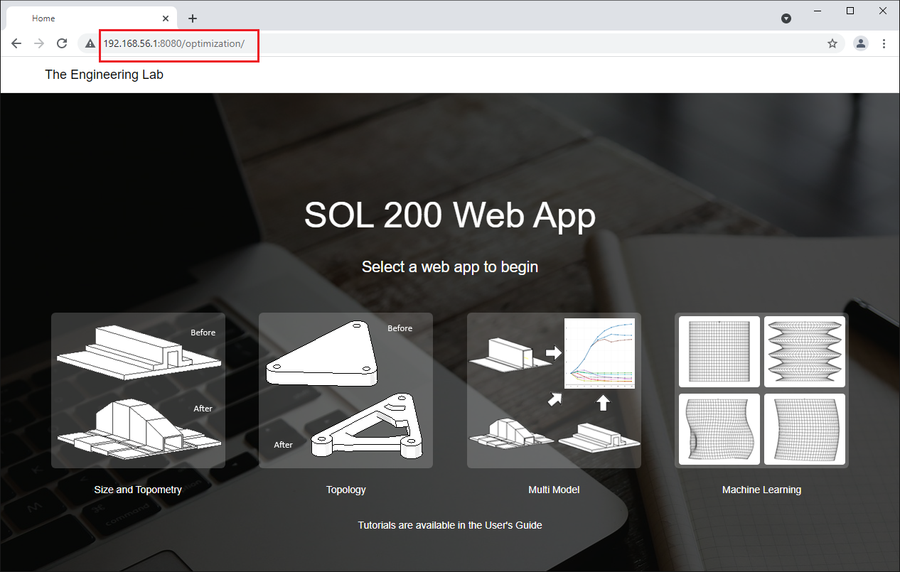
- You can close the command prompt to stop running the web app. To restart the web app again, repeat steps 6 and 7.
- If during the use of the SOL 200 Web App, you encounter messages indicating 0 available licenses,
this indicates the licensing is not correctly configured. Consider the following.
- Ensure you have followed the instructions to configure the license
- Contact technical support for assistance

How to automatically start the web app
Video Instructions
Instructions
- Open any folder on your desktop. Press the following key combination: ALT + V + Y + O .
This will open the Folder Options. Go to the View tab and uncheck 'Hide extensions for known file types.'
Click OK to close the Folder Options.
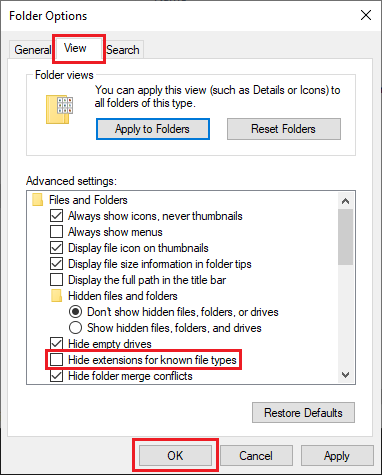
- Create a text file on your desktop and name it startup_app.bat. This batch (BAT) file will be use in the following steps.
- Add this text to the BAT file that was created.
Make sure to update the directory for your own web app
folder.
startup_app.batif not "%minimized%"=="" goto :minimized set minimized=true @echo off cd /D "C:\Users\caparici\Desktop\sol_200_web_app" start /min cmd /C "node app.min.js" goto :EOF :minimized - Right click on the BAT file and click Create shortcut. A new shortcut is created and named
startup_app.bat - Shortcut.
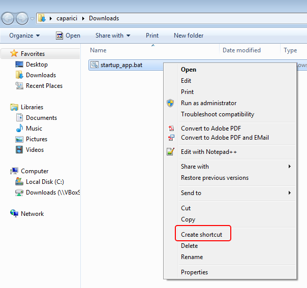
- Right click on the shortcut file
startup_app.bat - Shortcutand click Properties. A new Shortcut Properties window appears.
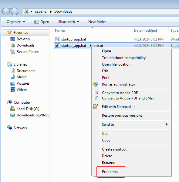
- Make the modifications as listed below.
- In the Shortcut Properties window, click Advanced.
- A new Advanced Properties window appears.
- Mark the checkbox for Run as administrator.
- Click OK on any open windows.
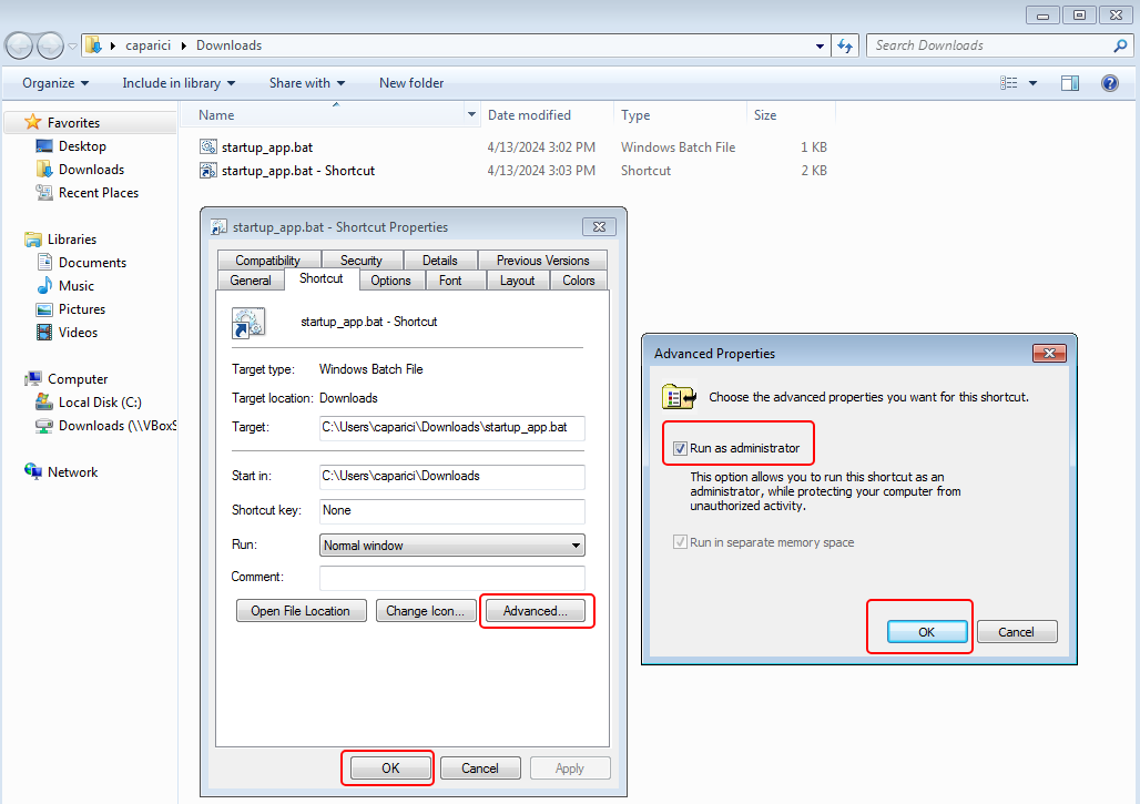
- The shortcut may now be used to start the web app. You can double click the shortcut and the SOL 200 Web App server will be started automatically.
Optionally, you can place the shortcut file in the 'Startup' folder so the server starts automatically when the machine is started. The location of the 'Startup' folder will vary for different versions of Windows. For some Windows operating systems, the ‘Startup’ folder is at this location, whereUSERNAMEis replaced with your actual username:C:\Users\USERNAME\AppData\Roaming\Microsoft\Windows\Start Menu\Programs\Startup
Enabling Web App Access to Other Devices
To access the web app from other machines on the network, follow this checklist. Instructions to complete this checklist are given further down.| Determine the IP Address of the Server | |
| Ping the Server | |
| Open and Verify Port 8080 of the Server is Open |
|
For demonstration purposes, it is assumed Computer A and B exist. It is very important to note that the IP addresses you work with will be different. Computer A (Server - The machine that hosts the web app)
|
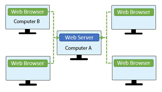
|
Determine the IP Address of the Server
Do the following on the server.
|
Output
C:\Users\User>ipconfig Windows IP Configuration Ethernet adapter Ethernet 2: Media State . . . . . . . . . . . : Media disconnected Connection-specific DNS Suffix . : Ethernet adapter Ethernet 3: Connection-specific DNS Suffix . : Link-local IPv6 Address . . . . . : fe80::a14d:b145:f240:50df%7 IPv4 Address. . . . . . . . . . . : 192.168.56.108 Subnet Mask . . . . . . . . . . . : 255.255.255.0 Default Gateway . . . . . . . . . : Ethernet adapter Ethernet 4: Connection-specific DNS Suffix . : Link-local IPv6 Address . . . . . : fe80::4495:1e84:f3c3:35e7%23 IPv4 Address. . . . . . . . . . . : 192.168.57.3 Subnet Mask . . . . . . . . . . . : 255.255.255.0 Default Gateway . . . . . . . . . : |
Ping the Server
The ping test is used to confirm if the address is accessible on the network.By default, Windows 10 is configured to ignore ping requests. These instructions enable ping requests.
Do the following on the server.
|
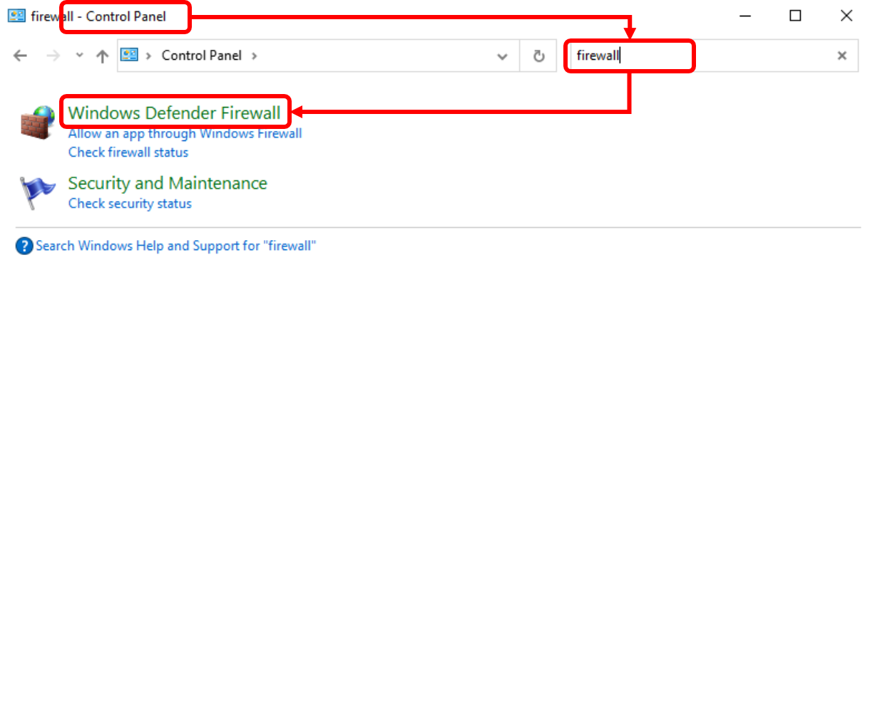
|
|
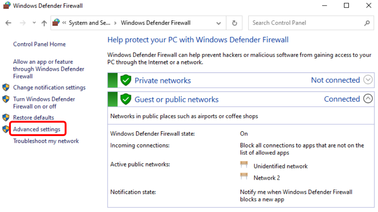
|
|
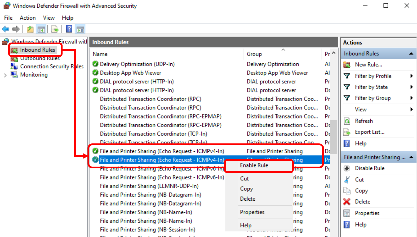
|
Do the following on the client.
|
Output
C:\Windows\system32>ping 192.168.56.108

Pinging 192.168.56.108 with 32 bytes of data:
Reply from 192.168.56.108: bytes=32 time=2ms TTL=128
Reply from 192.168.56.108: bytes=32 time<1ms TTL=128
Reply from 192.168.56.108: bytes=32 time=8ms TTL=128
Reply from 192.168.56.108: bytes=32 time<1ms TTL=128

Ping statistics for 192.168.56.108:
    Packets: Sent = 4, Received = 4, Lost = 0 (0% loss),
Approximate round trip times in milli-seconds:
    Minimum = 0ms, Maximum = 8ms, Average = 2ms
|
|
Output
C:\Windows\system32>ping 192.168.57.3

Pinging 192.168.57.3 with 32 bytes of data:
Request timed out.
Request timed out.
Request timed out.
Request timed out.

Ping statistics for 192.168.57.3:
    Packets: Sent = 4, Received = 0, Lost = 4 (100% loss),
|
Open and Verify Port 8080 of the Server is Open
To open port 8080, the following conditions must be fulfilled: First, the SOL 200 Web App must be running; Second, the firewall must be configured to open port 8080. Two methods are available to open port 8080.
Method 1
Do the following on the server.
|
Output
C:\Users\User\Desktop\nastran_sol_200_web_app_20210202_0944_v_5_0_0_beta>node app.min.js
Success! The SOL 200 Web App has started.
Desktop Version: Use Google Chrome and go to: http://localhost:8080/optimization
Network Version: Use Google Chrome and go to: http://IPADDRESS:8080/optimization
                 IPADDRESS is the IP address of this machine
                 Example: 192.168.56.102:8080/optimization
|
|
Output
PS C:\Users\User> Test-NetConnection -ComputerName 192.168.56.108 -Port 8080 WARNING: TCP connect to (192.168.56.108 : 8080) failed ComputerName : 192.168.56.108 RemoteAddress : 192.168.56.108 RemotePort : 8080 InterfaceAlias : Ethernet 3 SourceAddress : 192.168.56.108 PingSucceeded : True PingReplyDetails (RTT) : 0 ms TcpTestSucceeded : False |
|
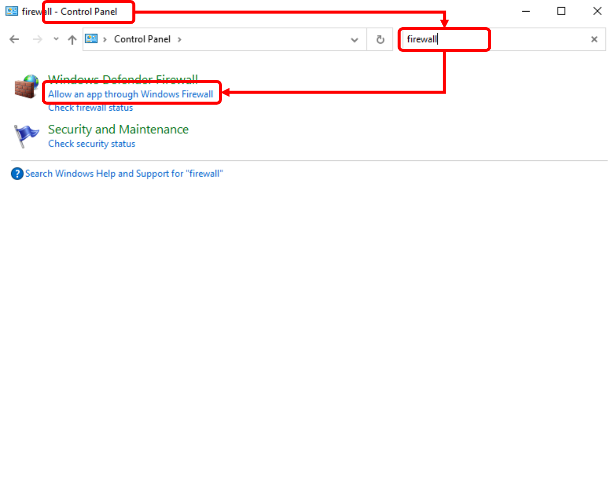
|
|
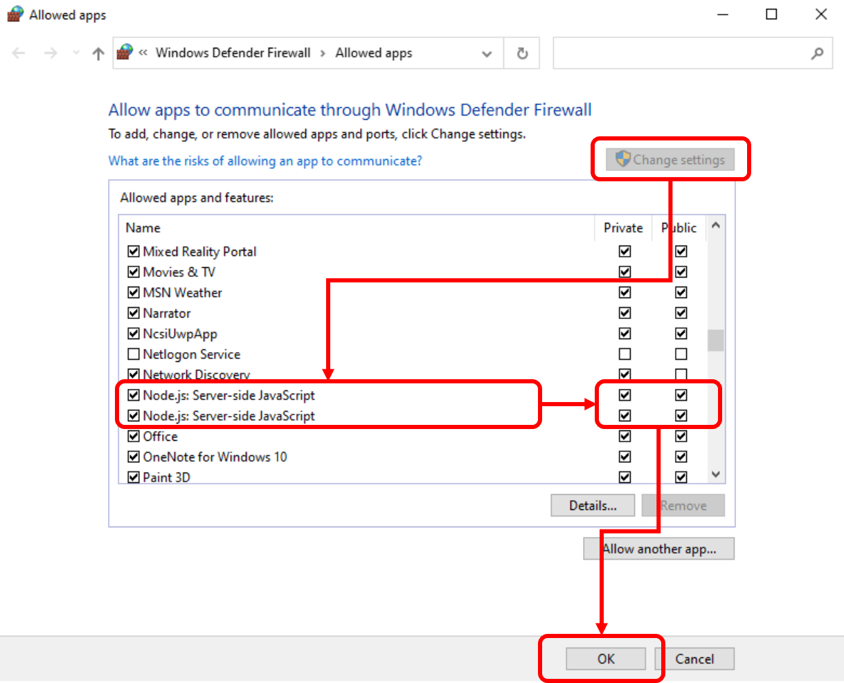
|
|
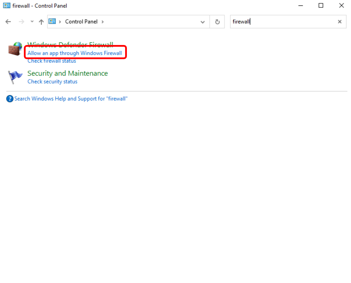
|
|
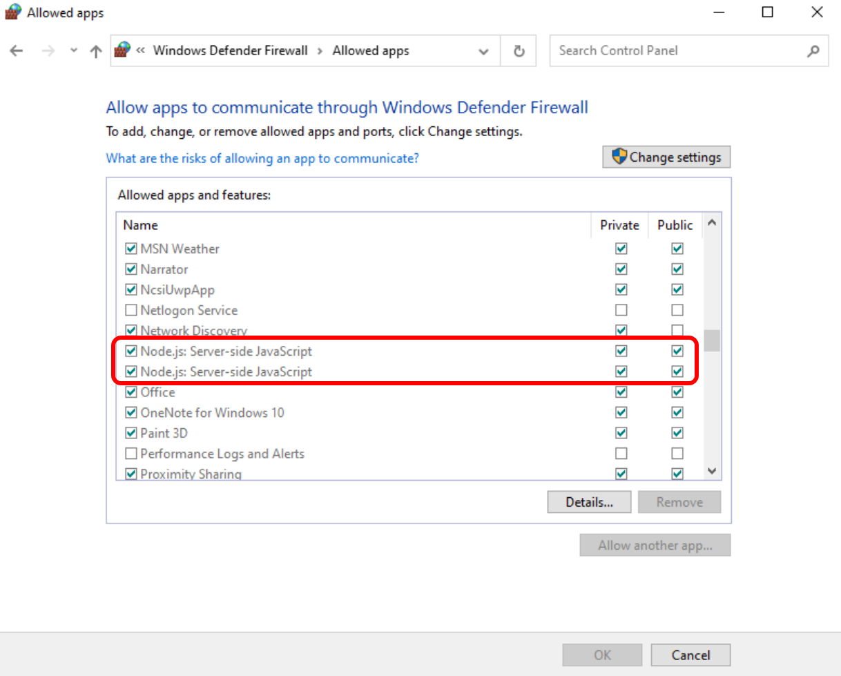
|
Do the following on the client.
|
Output
PS C:\Users\User> Test-NetConnection -ComputerName 192.168.56.108 -Port 8080 ComputerName : 192.168.56.108 RemoteAddress : 192.168.56.108 RemotePort : 8080 InterfaceAlias : Ethernet 3 SourceAddress : 192.168.56.108 TcpTestSucceeded : True |
|

|
Method 2
Do the following on the server.
|
Output
C:\Users\User\Desktop\nastran_sol_200_web_app_20210202_0944_v_5_0_0_beta>node app.min.js
Success! The SOL 200 Web App has started.
Desktop Version: Use Google Chrome and go to: http://localhost:8080/optimization
Network Version: Use Google Chrome and go to: http://IPADDRESS:8080/optimization
                 IPADDRESS is the IP address of this machine
                 Example: 192.168.56.102:8080/optimization
|
|
Output
PS C:\Users\User> Test-NetConnection -ComputerName 192.168.56.108 -Port 8080 WARNING: TCP connect to (192.168.56.108 : 8080) failed ComputerName : 192.168.56.108 RemoteAddress : 192.168.56.108 RemotePort : 8080 InterfaceAlias : Ethernet 3 SourceAddress : 192.168.56.108 PingSucceeded : True PingReplyDetails (RTT) : 0 ms TcpTestSucceeded : False |
|
|
|
|
|
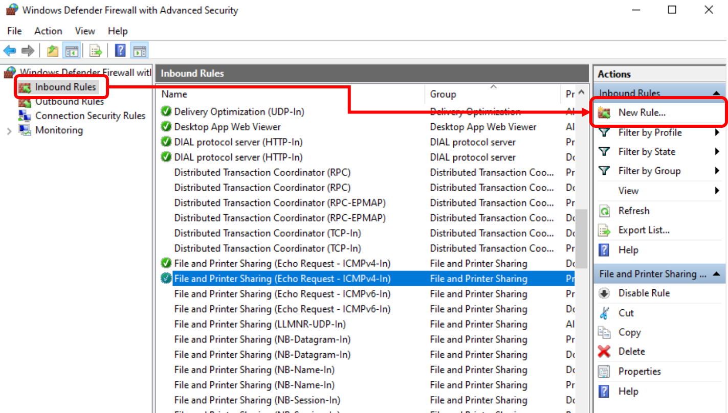
|
|
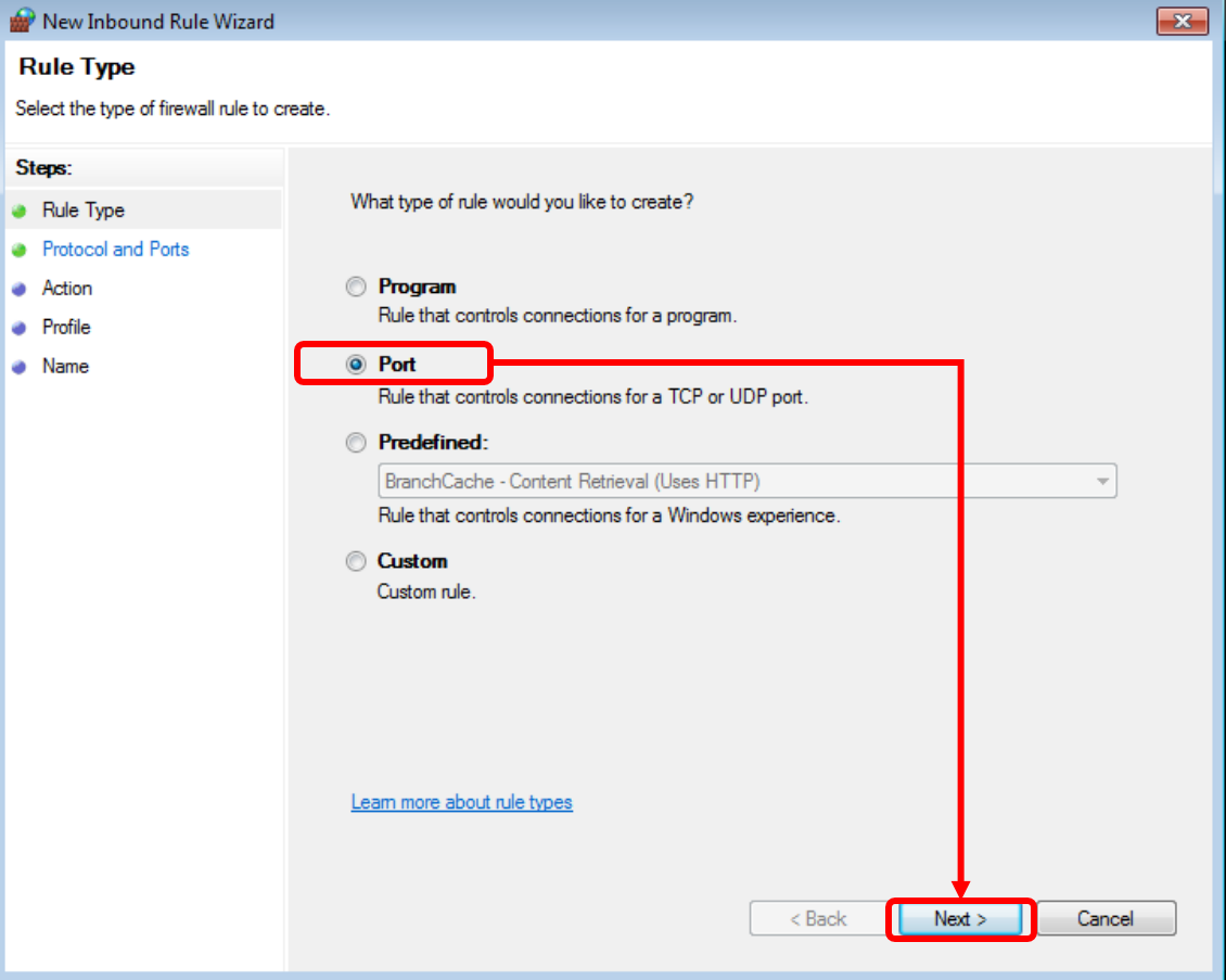
|
|
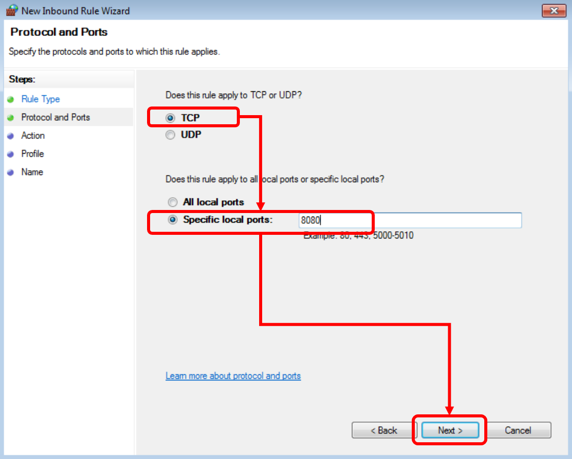
|
|
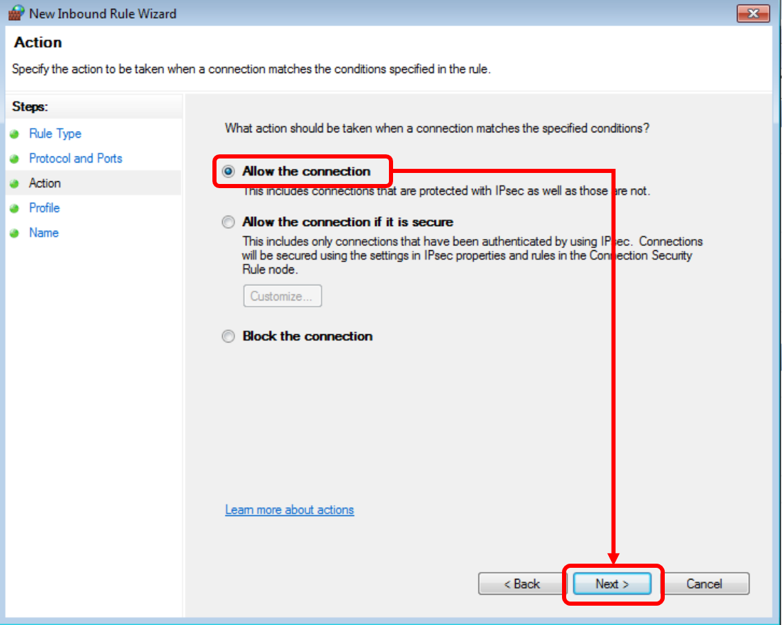
|
|
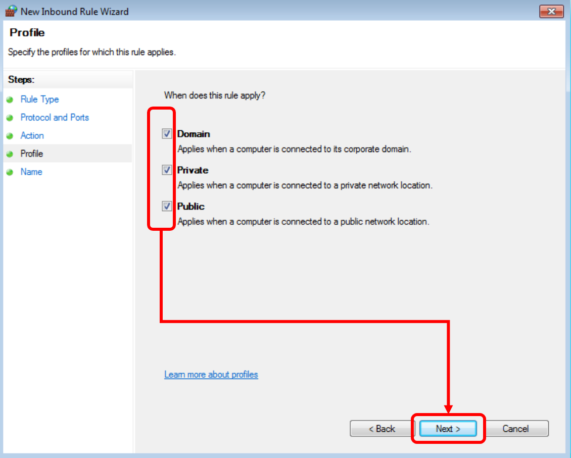
|
|
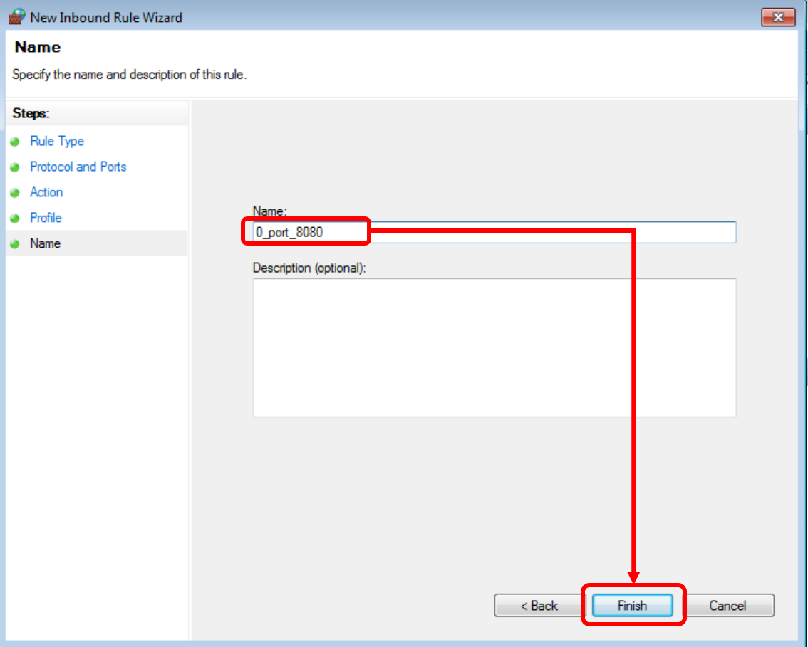
|
|
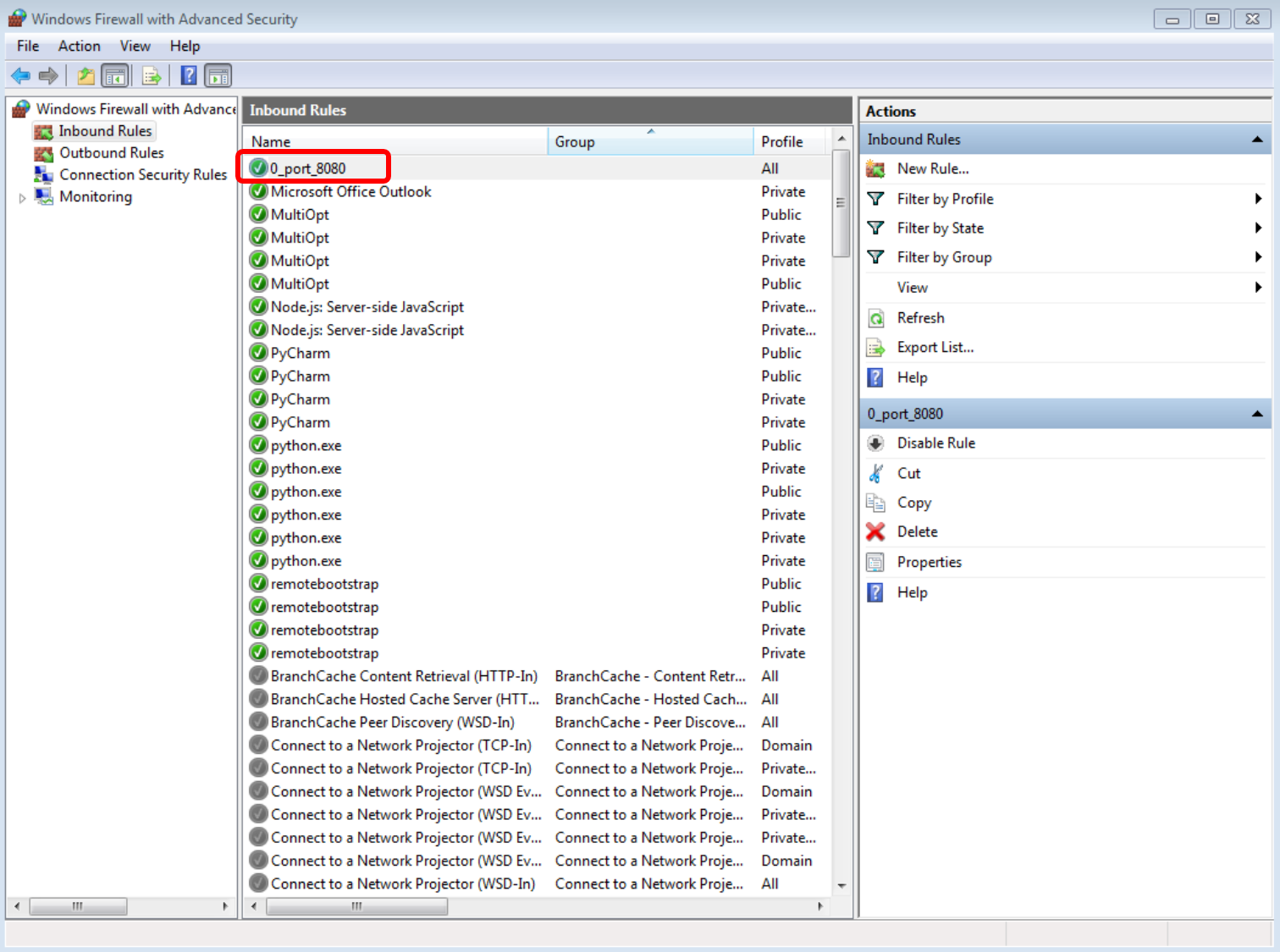
|
Do the following on the client.
|
Output
PS C:\Users\User> Test-NetConnection -ComputerName 192.168.56.108 -Port 8080 ComputerName : 192.168.56.108 RemoteAddress : 192.168.56.108 RemotePort : 8080 InterfaceAlias : Ethernet 3 SourceAddress : 192.168.56.108 TcpTestSucceeded : True |
|
|
Installation Procedure - Linux
The following are directions on how to install the SOL 200 Web App on Red Hat Enterprise
Linux (RHEL).
Video Instructions
Instructions
Prerequisites
- Ensure Google Chrome, Mozilla Firefox or Microsoft Edge is installed.
- Ensure 'sudo' privileges are available.
- Ensure Red Hat Enterprise Linux (RHEL) is registered and subscribed to access operating system updates.
- Ensure RHEL is connected to the network and has an IP address.
- Ensure the correct Network Device, e.g. enp0s8, enp0s3, is always enabled. In certain cases, the Network Device may be disabled on startup and will render the web app inaccessible.
The commands listed in this section are to be executed in the Terminal.
- Log in to the operating system using a non-root account.
-
It is highly recommended to use or create a separate user account with sudo
privileges when following these installation instructions. Do NOT use the
rootaccount for installation. -
Running any web server via the
rootaccount is not best practice. The following instructions configure a web server via Node JS and will make the SOL 200 Web App accessible to users on the local network.
-
It is highly recommended to use or create a separate user account with sudo
privileges when following these installation instructions. Do NOT use the
-
Download the web app
- Download the web app ZIP file, e.g. sol_200_web_app.zip .
- Extract the contents of the zip file to a folder named: sol_200_web_app .
- Licensing - To configure the licensing, following these instructions.
Method A - License File Prerequisites
You have been provided a license file, for example1100101101.dat.
Instructions- A.1 Ensure the license file name includes only the numbers 1 or 0 and the file extension '.dat' (Correct:
1100101101.datIncorrect:for_chris_1100101101.dat) - A.2 Take the license file (example: 10111010.dat) and put it in this directory
./sol_200_web_app/license
- A.1 Ensure the license file name includes only the numbers 1 or 0 and the file extension '.dat' (Correct:
- Install Node JS
Use Method 1 to install Node JS. If Method 1 does not work, Method 2 is an alternative method of installing Node JS.
Method 1 Method 2 Enable the Red Hat Software Collections (RHSCL) repository.
sudo yum-config-manager --enable rhel-server-rhscl-7-rpms
Execute this command to install Node JS.
sudo yum install rh-nodejs12
After installation, the Node JS software collection must be enabled. Do the following.
Create a new file
enablenodejs12.shin/etc/profile.d/sudo gedit /etc/profile.d/enablenodejs12.sh
Add the following text to file
enablenodejs12.sh.#!/bin/bash source scl_source enable rh-nodejs12
Use this to reload the settings. Alternatively, you may restart the system to reload the settings.
source /etc/profile.d/enablenodejs12.sh
Note: The command below also reloads the settings, but only for the current terminal window. If you open a new terminal window, the software collection will not be enabled. The command
scl enableis for short term use, but the fileenablenodejs12.shis for long term use.scl enable rh-nodejs12 bash
Add and enable NodeSource's Node.js repository
curl -sL https://rpm.nodesource.com/setup_12.x | sudo -E bash -
Execute this command to install Node JS.
sudo yum install -y nodejs
If an error regarding yum lock and PackageKit occurs, this command must be executed first.
sudo systemctl stop packagekit
Open a new Terminal window. To confirm Node JS has been installed, confirm that there is a version number that exists.
node --version
Example output. If a version number is displayed, then Node JS has been installed successfully. Continue to the next step.
node --version
v12.22.12
Important! Older versions of Node JS, such as version 6.17.1 are not compatible with the SOL 200 Web App.
Older versions may be removed with the terminal commands below.
If Red Hat Software Collections (RHSCL) was used to install Node JS, follow these instructions to remove Node JS.
# Remove Node JS
yum list installed | grep nodejs
sudo systemctl stop packagekit
sudo yum autoremove rh-nodejs6-runtime
yum list installed | grep nodejs

# Before
#     [user1@skynet ~]$ yum list installed | grep nodejs
#     rh-nodejs6.x86_64                    2.4-6.el7         @rhel-server-rhscl-7-rpms
#     rh-nodejs6-gyp.noarch                0.1-0.12.1617svn.el7
#     rh-nodejs6-http-parser.x86_64        2.7.0-4.el7       @rhel-server-rhscl-7-rpms
#     rh-nodejs6-http-parser-devel.x86_64  2.7.0-4.el7       @rhel-server-rhscl-7-rpms
#     rh-nodejs6-libuv.x86_64              1:1.9.1-3.el7     @rhel-server-rhscl-7-rpms
#     [...]
#     rh-nodejs6-nodejs-xtend.noarch       4.0.0-6.el7       @rhel-server-rhscl-7-rpms
#     rh-nodejs6-npm.noarch                3.10.9-3.el7      @rhel-server-rhscl-7-rpms
#     rh-nodejs6-runtime.x86_64            2.4-6.el7         @rhel-server-rhscl-7-rpms
#
# After (The rh-nodejs6 package is no longer listed)
#     [user1@skynet ~]$ yum list installed | grep nodejs
#
# Node JS may now be reinstalled
If NodeSource was used to install Node JS, follow these instructions to remove Node JS.
# First remove all Node JS repositories
cd /etc/yum.repos.d/
ls -l
sudo rm nodesource-el7.repo
sudo rm nodesource-el.repo
ls -l

# Before
#     [user1@skynet ~]$ ls -l
#     total 44
#     [...]
#     -rw-r--r--. 1 root root  616 Oct 23  2020 CentOS-x86_64-kernel.repo
#     -rw-r--r--. 1 root root  474 Apr 23  2019 nodesource-el7.repo
#     -rw-r--r--. 1 root root  474 Apr 23  2019 nodesource-el.repo
#
# After (Note the nodesource[...].repo lines are now removed)
#
#     [user1@skynet ~]$ ls -l
#     total 44
#     [...]
#     -rw-r--r--. 1 root root  616 Oct 23  2020 CentOS-x86_64-kernel.repo

# Remove Node JS
sudo yum remove nodejs  # Remove current Node JS
sudo yum clean all      # Purge any cached installation files, this step is important to avoid reinstalling cached and old installers
# Node JS may now be reinstalled
- Start the Web App
On the machine, navigate to this directory: ./sol_200_web_app
cd sol_200_web_app
Run this command to start the web app. The first start will ask you to accept the end user license agreement (EULA).
node app.min.js
If the location of the sol_200_web_app directory is restricted, sudo privileges will be required to start the web app.
sudo node app.min.js
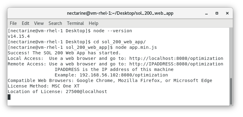
- Confirm the web app is Accessible
Open Google Chrome, Mozilla Firefox or Microsoft Edge and go to:
http://localhost:8080/optimization.If you can access the web app, this indicates the web app is running successfully.
The web app can be closed by closing the Terminal window or by pressing CTRL+C on the keyboard.
- Ensure executable files have execution privileges
The following files require execution privileges.
./sol_200_web_app/public/payload/app_design
./sol_200_web_app/public/payload/app_gp
./sol_200_web_app/public/payload/desktop_app_a
Use these commands in the terminal to give execution privileges to these files.
cd sol_200_web_app/public/payload
chmod ugo+x app_design
chmod ugo+x app_gp
chmod ugo+x desktop_app_a
cd ../../..
This command may be used to confirm the files have execution privileges.
ls -l sol_200_web_app/public/payload
Example Output - Note that the presence of x characters indicates the files have execution privileges.
[nectarine@vm-rhel-1 Desktop]$ ls -l sol_200_web_app/public/payload
total 697900
-rwxr-xr-x. 1 nectarine nectarine  57769440 Jul 27 09:59 app_design
-rw-rw-r--. 1 nectarine nectarine  54931899 Jul 27 09:59 app_design.exe
-rwxr-xr-x. 1 nectarine nectarine  89722536 Jul 27 09:59 app_gp
-rw-rw-r--. 1 nectarine nectarine  79401492 Jul 27 09:59 app_gp.exe
-rwxrwxr-x. 1 nectarine nectarine  33392072 Jul 27 09:59 desktop_app_a
-rw-rw-r--. 1 nectarine nectarine  24646867 Jul 27 09:59 desktop_app_a.exe
[...]
- If during the use of the SOL 200 Web App, you encounter messages indicating 0 available licenses,
this indicates the licensing is not correctly configured. Consider the following.
- Ensure you have followed the instructions to configure the license
- Contact technical support for assistance
-
Open Port 8080
For the remainder of this guide, "machine" will be referred to the workstation or server that has the SOL 200 Web App installed. Any variation of "machine" such as "second machine" is a different workstation or server.
By default, RHEL will have port 8080 closed. The following commands will open port 8080. Note that the SOL 200 Web App is configured to use only port 8080.
On the machine, uses these commands to open port 8080.
$ sudo firewall-cmd --list-ports

$ sudo firewall-cmd --zone=public --add-port=8080/tcp --permanent
success
$ sudo firewall-cmd --reload
success
After these commands are executed, listing the ports now shows port 8080 is opened for TCP.
Note: If
8080/tcpis not listed, the machine must be restarted for the changes to take effect.$ sudo firewall-cmd --list-ports 8080/tcp
- Confirm the web app is Accessible
On a different machine, open Google Chrome, Mozilla Firefox or Microsoft Edge and go to:
http://IPADDRESS:8080/optimization. Note that theIPADDRESSshould be the IP of the machine that has the sol_200_web_app directory. Examples:- http://172.31.99.137:8080/optimization
- http://192.168.1.234:8080/optimization
If you can access the web app, the web is now accessible by other machines on the network.
- Set the web app to run in the background
Process Manager 2 (PM2) will be used to automatically run the SOL 200 Web App in the background. PM2 also automatically starts the SOL 200 Web App after the operating system is restarted.
Important! Before continuing, please keep consider the following.
-
Be sure that the SOL 200 Web App is working successfully when using
node app.min.jsto start the web app. To verify the SOL 200 Web App is functioning properly, perform at least one tutorial listed in the Tutorials section. -
If the SOL 200 Web App is currently running via
node app.min.jsin a terminal, please stop this process by pressing CTRL+C or by closing the terminal window.
The following are instructions to configure the SOL 200 Web App to run in the background.
Install PM2 using this command.
sudo npm install pm2 -g
Use this command to generate output. The output is used in the next step.
pm2 startup
The output will give you a new command to use. Execute this command. Note, your command may be slightly different. This command will add PM2 to the list of startup process on the system.
sudo env PATH=$PATH:/usr/bin /usr/lib/node_modules/pm2/bin/pm2 startup systemd -u apricot --hp /home/apricot
Navigate to the location of the
ecosystem.config.jsonfile and use PM2 to start the web app.cd /home/apricot/Downloads/sol_200_web_app pm2 start ecosystem.config.json
Use this command to save the web app to the list of startup applications in PM2.
pm2 save
Open Google Chrome, Mozilla Firefox or Microsoft Edge and go to:
http://IPADDRESS:8080/optimization. Note that theIPADDRESSshould be the IP of your RHEL server. Examples:- http://172.31.99.137:8080/optimization
- http://192.168.1.234:8080/optimization
If you can access the web app, PM2 has been properly configured to automatically run the SOL 200 Web App in the background when the system is restarted.
To confirm the SOL 200 Web App is automatically running after the operating system is restarted, do the following. Restart the operating system at your convenience. Open a web browser and confirm you can access the SOL 200 Web App. If successful, this confirms the SOL 200 Web App is running in the background after the system is restarted.
PM2 ExamplesBelow are more explicit PM2 examples. These examples start off assuming the SOL 200 Web App has not yet been configured with PM2.
Inspect the current list of processes being managed by PM2.
$ pm2 list all
[PM2] Spawning PM2 daemon with pm2_home=/home/apricot/.pm2
[PM2] PM2 Successfully daemonized
┌────┬────────────────────┬──────────┬──────┬───────────┬──────────┬──────────┐
│ id │ name               │ mode     │ ↺    │ status    │ cpu      │ memory   │
└────┴────────────────────┴──────────┴──────┴───────────┴──────────┴──────────┘
The output indicates there are no processes being managed by PM2.
Navigate to the SOL 200 Web App directory.
$ cd ./sol_200_web_app/
Now use PM2 to start the SOL 200 Web App by using the configuration file
ecosystem.config.json. This JSON file contains information to start the SOL 200 Web App.$ pm2 start ecosystem.config.json [PM2][WARN] Applications sol_200_web_app not running, starting... [PM2] App [sol_200_web_app] launched (1 instances) ┌────┬────────────────────┬──────────┬──────┬───────────┬──────────┬──────────┐ │ id │ name │ mode │ ↺ │ status │ cpu │ memory │ ├────┼────────────────────┼──────────┼──────┼───────────┼──────────┼──────────┤ │ 0 │ sol_200_web_app │ fork │ 0 │ online │ 0% │ 20.6mb │ └────┴────────────────────┴──────────┴──────┴───────────┴──────────┴──────────┘
The outputted table shows the process named
sol_200_web_apphas started and its status is online.Save the edits made. Any time a start, stop or delete command is performed, a save must be done afterwards.
$ pm2 save
[PM2] Saving current process list...
[PM2] Successfully saved in /home/apricot/.pm2/dump.pm2
The terminal window may now be closed and PM2 will keep the SOL 200 Web App running in the background. If the system is restarted, PM2 will automatically restart the SOL 200 Web App on the next system startup.
At any time, the log files of the
sol_200_web_appprocess may be inspected.$ pm2 logs sol_200_web_app [TAILING] Tailing last 15 lines for [sol_200_web_app] process (change the value with --lines option) /home/apricot/.pm2/logs/sol-200-web-app-error.log last 15 lines: /home/apricot/.pm2/logs/sol-200-web-app-out.log last 15 lines: 0|sol_200_ | Success! The SOL 200 Web App has started. 0|sol_200_ | Local Access: Use a web browser and go to: http://localhost:8080/optimization 0|sol_200_ | Remote Access: Use a web browser and go to: http://IPADDRESS:8080/optimization 0|sol_200_ | IPADDRESS is the IP address of this machine 0|sol_200_ | Example: 192.168.56.102:8080/optimization 0|sol_200_ | Compatible Web Browsers: Google Chrome, Mozilla Firefox, or Microsoft Edge 0|sol_200_ | License Method: DAT File
This output is updated automatically. To exit the view of the logs, press CTRL+C or close the terminal window. Recall that PM2 will keep the sol_200_web_app process running in the background.
To clear the log files, use this command.
$ pm2 flush
[PM2] Flushing /home/apricot/.pm2/pm2.log
[PM2] Flushing:
[PM2] /home/apricot/.pm2/logs/sol-200-web-app-out.log
[PM2] /home/apricot/.pm2/logs/sol-200-web-app-error.log
[PM2] Logs flushed
This command is used to list all the existing processes managed by PM2.
$ pm2 list all
┌────┬────────────────────┬──────────┬──────┬───────────┬──────────┬──────────┐
│ id │ name               │ mode     │ ↺    │ status    │ cpu      │ memory   │
├────┼────────────────────┼──────────┼──────┼───────────┼──────────┼──────────┤
│ 0  │ sol_200_web_app    │ fork     │ 0    │ online    │ 0%       │ 63.2mb   │
└────┴────────────────────┴──────────┴──────┴───────────┴──────────┴──────────┘
The output indicates one process named
sol_200_web_appis currently online and running.This command is used to stop the SOL 200 Web App.
$ pm2 stop sol_200_web_app
[PM2] Applying action stopProcessId on app [sol_200_web_app](ids: [ 0 ])
[PM2] [sol_200_web_app](0) ✓
┌────┬────────────────────┬──────────┬──────┬───────────┬──────────┬──────────┐
│ id │ name               │ mode     │ ↺    │ status    │ cpu      │ memory   │
├────┼────────────────────┼──────────┼──────┼───────────┼──────────┼──────────┤
│ 0  │ sol_200_web_app    │ fork     │ 0    │ stopped   │ 0%       │ 0b       │
└────┴────────────────────┴──────────┴──────┴───────────┴──────────┴──────────┘
After performing a start, stop or delete, the current configuration must be saved. If you do not perform a save, the next time the operating system is restarted, PM2 will restart the
sol_200_web_appprocess even though you performed a stop before. Be sure to save.$ pm2 save [PM2] Saving current process list... [PM2] Successfully saved in /home/apricot/.pm2/dump.pm2
To permanently remove the SOL 200 Web App from being managed by PM2, execute a delete command.
$ pm2 delete sol_200_web_app
[PM2] Applying action deleteProcessId on app [sol_200_web_app](ids: [ 0 ])
[PM2] [sol_200_web_app](0) ✓
┌────┬────────────────────┬──────────┬──────┬───────────┬──────────┬──────────┐
│ id │ name               │ mode     │ ↺    │ status    │ cpu      │ memory   │
└────┴────────────────────┴──────────┴──────┴───────────┴──────────┴──────────┘
[PM2][WARN] Current process list is not synchronized with saved list. App sol_200_web_app differs. Type 'pm2 save' to synchronize.
Remember to save after a start, stop or delete command. If a delete command is performed, the force option must be used.
$ pm2 save --force
[PM2] Saving current process list...
[PM2] Successfully saved in /home/apricot/.pm2/dump.pm2
Confirm the sol_200_web_app process has been removed.$ pm2 list all ┌────┬────────────────────┬──────────┬──────┬───────────┬──────────┬──────────┐ │ id │ name │ mode │ ↺ │ status │ cpu │ memory │ └────┴────────────────────┴──────────┴──────┴───────────┴──────────┴──────────┘
Updating PM2 to Use a Newer Version of the SOL 200 Web AppPM2 may run only one version of the SOL 200 Web App (web app). If there is a need to use a different version of the web app, the previous web app version must be stopped and removed. The stop and removal process is detailed in this section.
Before starting, ensure the newest version of the web app functions properly via the command below. Consider going through at least one exercise in the Tutorials section to confirm the web app is functioning properly.
node app.min.js
After the web app is confirmed to be working with the above command, you may stop the web app by closing the terminal window or pressing CTRL+C to stop the web app.
The following describes how PM2 is used to replace older versions of the web app.
First, stop and delete the sol_200_web_app process. Save the changes afterwards.
pm2 stop sol_200_web_app
pm2 delete sol_200_web_app
pm2 save --force
Navigate to the newest location of the web app. Your location will differ. Start the web app like normal and save the newest process.
cd ./sol_200_web_app_newer_version
pm2 start ecosystem.config.json
pm2 save
The newest web app should now be running. Open a web browser to access the web app.
If at anytime, you would like to switch back to starting the web app with
node app.min.js, you must stop and delete the sol_200_web_app process.pm2 stop sol_200_web_app pm2 delete sol_200_web_app pm2 save --force
Removing PM2The following instructions describes how to completely remove PM2 from the system.
First inspect the global packages currently installed.
$ npm -g ls
Consider the output of the command above. Before removal, one of the listed installed packages is pm2.
/usr/lib
├── corepack@0.10.0
├─┬ npm@6.14.17
│ ├── abbrev@1.1.1
│ ├── ansicolors@0.3.2
│ [...]
└─┬ pm2@5.2.0
  ├─┬ @pm2/agent@2.0.1
  │ ├── async@3.2.4 deduped
To begin the removal of PM2, the PM2 process must first be removed from the operating system's list of startup processes. Execute this command in a terminal.
pm2 unstartup
The command above yields an output similar to below, your output will be different. Execute the outputted command in the terminal.
sudo env PATH=$PATH:/usr/bin /usr/lib/node_modules/pm2/bin/pm2 unstartup systemd -u apricot --hp /home/apricot
To finish removal of PM2, remove the PM2 package with this command.
sudo npm -g rm pm2
Verify pm2 has been removed with this command.
$ npm -g ls
The output of the command should look similar to this. Note that pm2 is no longer listed, indicating pm2 has been successfully removed.
/usr/lib
├── corepack@0.10.0
└─┬ npm@6.14.17
  ├── abbrev@1.1.1
  ├── ansicolors@0.3.2
  [...]
PM2 CommandsBelow is a short list of PM2 commands used in this documenation.
pm2 delete|del [id|name|all]          stop and delete a process from pm2 process list
pm2 flush [name]                      flush logs
pm2 list|ls                           list all processes
pm2 logs [id|name]                    stream logs file. Default stream all logs
pm2 restart [id|name|all]             restart a process
pm2 save|dump [options]               dump all processes for resurrecting them later
pm2 stop [options] [id|name|all]      stop a process
-
Be sure that the SOL 200 Web App is working successfully when using