What is the SOL 200 Web App?
The SOL 200 Web App is a collection of optimization and machine learning web apps, all with the purpose of improving the performance of MSC Nastran models.
Compatibility- Supported Web Browsers: Google Chrome, Mozilla Firefox or Microsoft Edge
- Supported Operating Systems: Windows and Red Hat Linux
- The SOL 200 Web App may be installed on a laptop, workstation or server. All data remains within your company.
SOL 200 Web App Capabilities
A datasheet is available with the free trial or on request.
List of Available Web Apps| Web App | SOL 200 Web App | Pre/Post Web App |
|---|---|---|
| Optimization Web App for MSC Nastran SOL 200 | ✔ | |
| Multi-model Optimization Web App | ✔ | |
| Machine Learning Web App | ✔ | |
| Shape Optimization Web App | ✔ | |
| Topology Optimization Web App | ✔ | |
| Composite Optimization Web App | ✔ | |
| Stacking Sequence Optimization Web App | ✔ | |
| Remote Execution Web App | ✔ | |
| PBMSECT/PBRSECT Web App | ✔ | |
| Dynamics Loads (RLOAD1/RLOAD2) Web App | ✔ | |
| Pre-processor Web App to configure MSC Nastran input files | ✔ | ✔ |
| Post-processor Web App to view MSC Nastran results | ✔ | ✔ |
| HDF5 Explorer to create graphs (XY plots) of MSC Nastran results | ✔ | ✔ |
| Uncertainty Quantification Results Web App | ✔ |
New Web Apps
| Web App Name | Link | Description |
|---|---|---|
| DMI Web App | Link | The Nastran stiffness matrix, mass matrix or other matrices may be exported to a punch file (.pch) and stored in DMI or DMIG bulk data entries. The DMI web app converts these DMI or DMIG entries to a CSV file. The Nastran stiffness matrix, mass matrix and other matrices stored in the CSV file maybe opened in Excel or other spreadsheet applications. |
About The Engineering Lab
The Engineering Lab's mission is to enable engineers worldwide with the web applications and training necessary to use optimization and machine learning methods to improve the performance of structural and mechanical systems.
What does The Engineering Lab do?
- Web Apps for Optimization and Machine Learning - The Engineering Lab develops web applications that enable engineers to optimize finite element models with either gradient-based optimizers or machine learning technology. The primary finite element analysis solver supported is MSC Nastran.
- Training for Optimization and Machine Learning - The Engineering Lab offers training lectures and tutorials detailing the necessary steps to utilize MSC Nastran's optimizer or machine learning technology. With training provided by The Engineering Lab, engineers will be better prepared to use the latest computational methods to improve the performance of structural and mechanical systems.
- Custom Web Apps for Engineers - The Engineering Lab builds custom web applications for engineers. These custom web apps are built using the latest web development methods and are rapidly deployed to meet a broad range of requirements. Examples include custom user interfaces to FE solvers, desktop automation, simulation results processing and more. Contact The Engineering Lab today to inquire about your custom web application.
Inquiries may be forwarded to christian@ the-engineering-lab.com.

Nastran SOL 200 Tutorials
Over 75 step-by-step tutorials are available regarding fundamentals of optimization and how to properly use the SOL 200 Web App. Click on any of the following links to jump to the section.
- Basic Optimization Tutorials
- Size Optimization Tutorials
- Topology, Topometry and Topography Tutorials
- Advanced Optimization Tutorials
- Miscellaneous Tutorials
- Machine Learning Tutorials
- Beams Tutorials
- Composite Laminate Optimization Tutorials
- Shape Optimization Tutorials
- Post-processor Tutorials
- Uncertainty Quantification Tutorials
- Optimization Under Uncertainty Tutorials
- Presentations
Please contact christian@ the-engineering-lab.com if you are interested in further Nastran SOL 200 guidance or training.
Basic Optimization Tutorials
| Title and Description | YouTube Tutorial | |
|---|---|---|
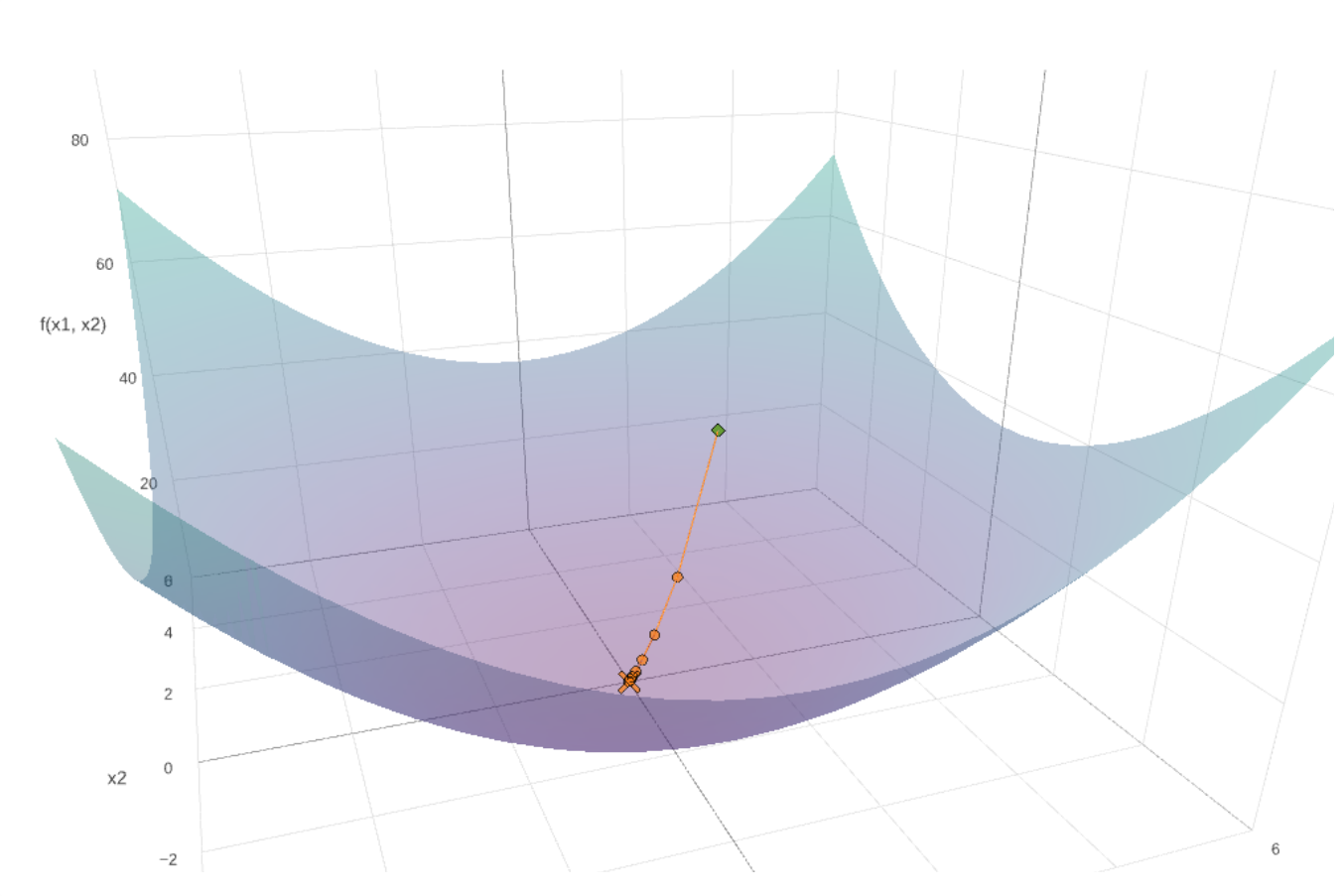 |
Unconstrained Optimization with MSC Nastran SOL 200 Part of Calculus involves finding maximums or minimums of functions. The process of finding maximums or minimums is the essence of optimization. In this video, MSC Nastran Optimization is used to find the optimum point or minimum of a two-variable function, f(y1, y2) = y1^2 + y2^2. |
Link |
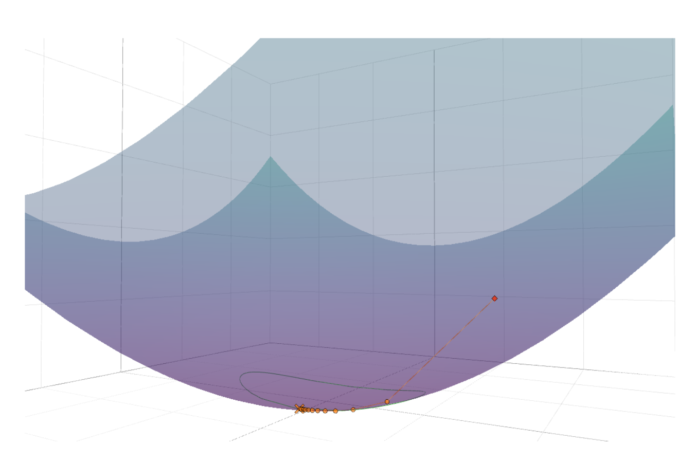 |
Constrained Optimization with MSC Nastran SOL 200 This video demonstrates the use of MSC Nastran Optimization to find the minimum of f(y1, y2) subject to a constraint g(y1, y2). |
Link |
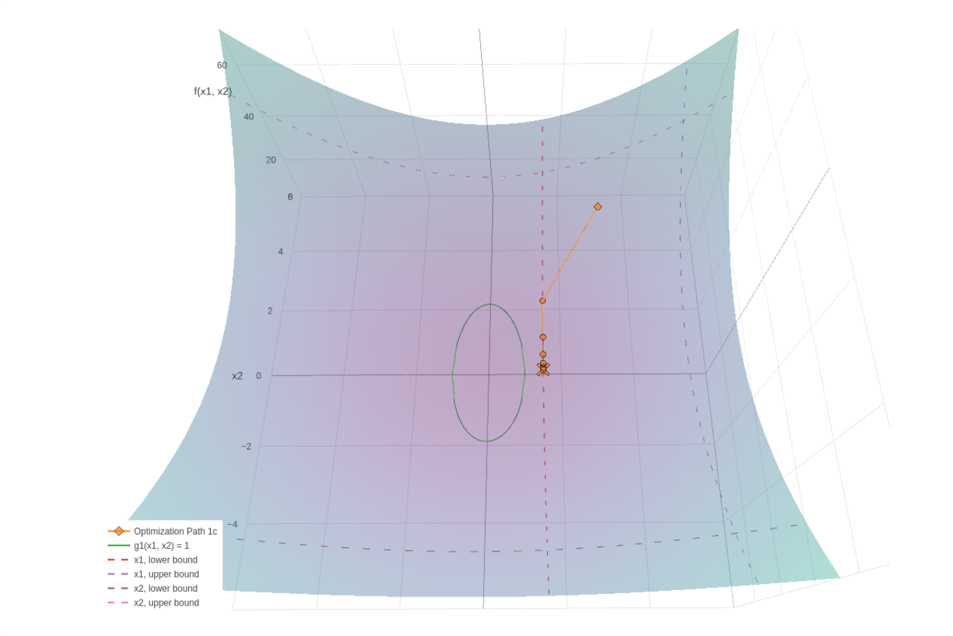 |
Side Constraints on Design Variables - MSC Nastran Optimization This video demonstrates the use of MSC Nastran Optimization to find the minimum of f(y1, y2) subject to limits on the design variables y1 and y2. |
Link |
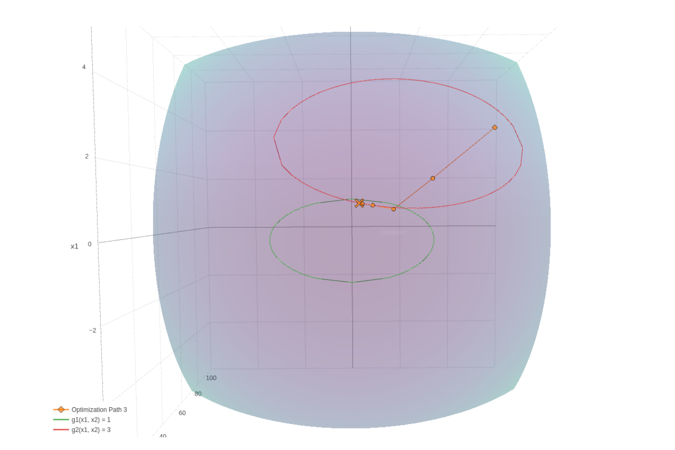 |
Best Compromise Infeasible Design - MSC Nastran Optimization In constrained optimization, an optimum solution may not exist that satisfies all the constraints. This video demonstrates such a scenario and walks through a fix. |
Link |
 |
What is Global Optimization? MSC Nastran SOL 200 / Optimization Tutorial This video discusses the meaning of Global Optimization and walks you through the process of setting up a Global Optimization with MSC Nastran SOL 200. |
Link |
 |
What is size optimization? What is shape, topology, topography and topometry optimization? In this short video, the following MSC Nastran optimization types are described.
|
Link |
Size Optimization Tutorials
| Title and Description | Lecture Notes | PDF Tutorial | YouTube Tutorial | |
|---|---|---|---|---|
 |
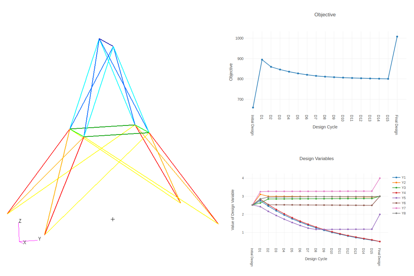
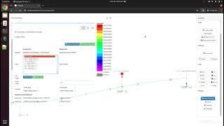
Structural Optimization of a 3 Bar Truss - MSC Nastran Optimization A truss structure is optimized with MSC Nastran. The design variables are the cross-sectional areas of the rod elements. The objective is to minimize the weight of the structure while ensuring the stress and displacements are within specified constraints. Starting BDF Files: Link Solution BDF Files: Link |
Link | Link | Link |
 |
Sensitivity Analysis of a 3 Bar Truss - MSC Nastran Optimization A structural optimization was previously performed on a 3 bar truss. In this tutorial, the process to perform a sensitivity analysis is detailed. Starting BDF Files: Link Solution BDF Files: Link |
Link | Link | |
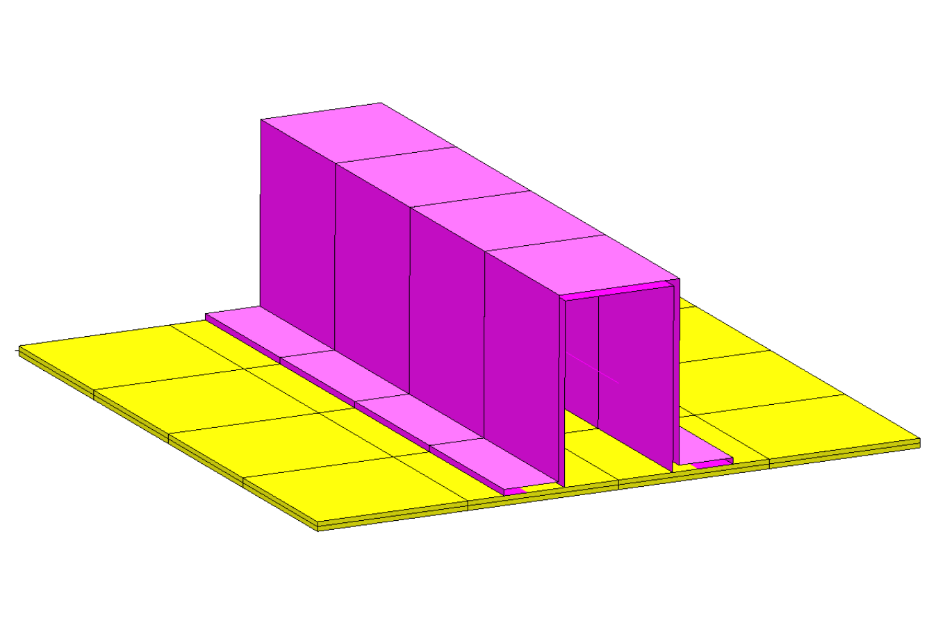 |
Automated Structural Optimization of a Stiffened Plate with MSC Nastran SOL 200/Design Optimization This example demonstrates the use of MSC Nastran to optimize the thickness of the plate and the thickness of a beam section to minimize weight. Constraints are imposed on the stresses in the shell and beam elements. Additional constraints are imposed on deflections. Starting BDF Files: Link Solution BDF Files: Link |
Link | Link | Link |
 |
Vibration of a Cantilevered Beam (Turner's Problem), MSC Nastran Optimization This example demonstrates the use of MSC Nastran to optimize the rod areas and shell thicknesses such that the structure's weight is minimized and the first natural frequency is above 20 Hz. Starting BDF Files: Link Solution BDF Files: Link |
Link | Link | Link |
 |
Dynamic Response Optimization with MSC Nastran Optimization This example is from the MSC Nastran Design Sensitivity and Optimization User's Guide. Starting BDF Files: Link Solution BDF Files: Link |
Link | Link | Link |
 |
Model Matching, Frequency Response Analysis A frequency response analysis has been performed, but the results do not match experimental results. This tutorial discusses the model matching procedure in order to correlate Finite Element Analysis and test results. Starting BDF Files: Link Solution BDF Files: Link |
Link | Link | |
 |
Using MSC Nastran Optimization for Model Matching / System Identification In this example, the cross section of a rod is designed such that the analysis modes match experimentally measured data. MSC Nastran Optimization is used to minimize the root sum of squares for Mode 1. This example is an adaptation of the example found in the UAI/Nastran User's Guide for Version 20.1 - 252.6.6 System Identification. The following is an excerpt from the guide describing this example. Keep in mind this video is an adaptation and will not match all the values in the following description: Starting BDF Files: Link Solution BDF Files: Link |
Link | Link | Link |
 |
Ply Number Optimization of a Composite Laminate with MSC Nastran Optimization (SOL 200) This tutorial details the process to configure a ply number optimization for MSC Nastran. The optimization problem statement is to reduce the mass of a composite cylinder, ensure ply failure index constraints are satisfied, and vary the number of plies for 0, 90 and +/-45-degree layers. This example considers ply number optimization for multiple PCOMP entries and multiple load cases. Additional comments are made regarding displaying fringe plots of the failure indices after optimization, updating the final BDF files with new PCOMP entries, and stacking sequence optimization. Starting BDF Files: Link Solution BDF Files: Link |
Link | Link | |
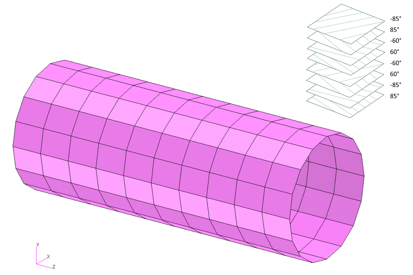 |
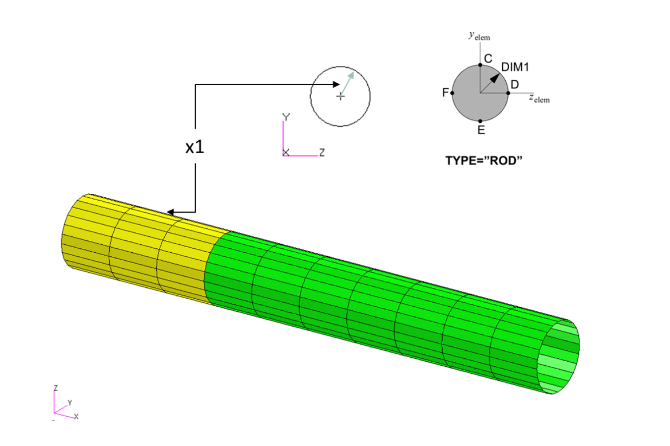
Automated Optimization of a Composite Laminate with MSC Nastran Optimization (SOL 200) This example details the use of MSC Nastran Design Optimization (SOL 200) to optimize the weight of a tube composed of a composite laminate. The ply thicknesses and orientations are allowed to vary during the optimization process. The orientation angles are limited to 5 degree increments. Constraints on the failure indices are applied. Starting BDF Files: Link Solution BDF Files: Link |
Link | Link | Link |
 |
Optimizing for Buckling - Twenty-Five Bar Truss with MSC Nastran Optimization This example is from the MSC Nastran Design Sensitivity and Optimization User's Guide.
Starting BDF Files: Link Solution BDF Files: Link |
Link | Link | Link |
 |
Acoustic Optimization, Beta Method A fluid is enclosed in a structural box and subjected to an acoustic source. The goal is to minimize the peak acoustic pressure while letting the structural thicknesses vary and preventing the weight from significantly changing. Starting BDF Files: Link Solution BDF Files: Link |
Link | Link | Link |
 |
Acoustic Optimization, Nastran BETA Function This tutorial is a repeat of the previous Acoustic Optimization example, but highlights an alternative method to setting up the optimization for Nastran SOL 200. The BETA method is used and reduces the work that was previously required. Starting BDF Files: Link Solution BDF Files: Link |
Link | Link | |
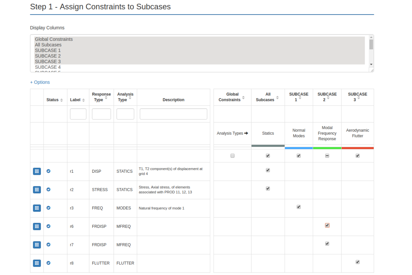 |
Optimization for Multiple Load Cases or SUBCASEs The web app makes simple configuring design constraints for dozens or hundreds of load cases. This tutorial guides you through the process. Starting BDF Files: Link Solution BDF Files: Link |
Link | Link | |
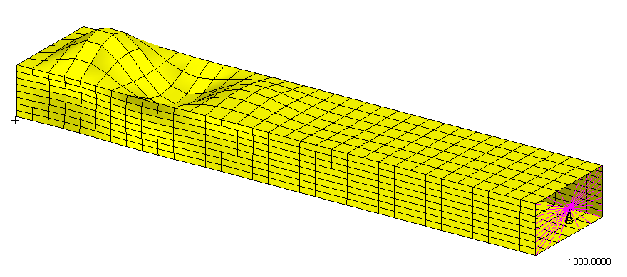 |
Buckling Optimization of a Cantilever Beam This example demonstrates the procedure to configure Nastran SOL 200 for buckling optimization. This example also covers how to optimize for multiple buckling scenarios. Starting BDF Files: Link Solution BDF Files: Link |
Link | Link | |
|
Global Optimization This example demonstrates the procedure of performing a Global Optimization with MSC Nastran SOL 200. Often, optimization problems have multiple local minimums, or maximums, when starting from different initial design variables. To find the global optimum, multiple local optimizations must be performed, then the best of the local optimizations is taken to be global optimum. This process can be performed with the Global Optimization capability available in MSC Nastran SOL 200. Starting BDF Files: Link Solution BDF Files: Link |
Link | Link | |
|
Parameter Study This tutorial details the use of MSC Nastran SOL 200 to perform a "parameter study." What is a parameter study? A common engineering technique is to try different structural configurations, for example, changing structural dimensions, and review the impact on structural responses such as displacements and stresses. Dozens, possibly hundreds of structural configurations would ideally be evaluated. This is termed "parameter study." MSC Nastran SOL 200 includes a capability to automatically generate multiple structural configurations and perform static or dynamic analyses. The outcome are results from multiple structural configurations that can be compared. Starting BDF Files: Link Solution BDF Files: Link |
Link | Link | |
 |
Multi Model Optimization Multi Model Optimization (MMO) is the process of optimizing multiple design models concurrently. Design variables across multiple models can be linked and simultaneously optimized. A merged or combined objective can optimize the objective of each design model. The design constraints of each design model are also included in a multi model optimization. This tutorial details the procedure to configure a multi model optimization. Starting BDF Files: Link Solution BDF Files: Link |
Link | Link |
Topology, Topometry and Topography Optimization Tutorials
| Title and Description | Lecture Notes | PDF Tutorial | YouTube Tutorial | |
|---|---|---|---|---|
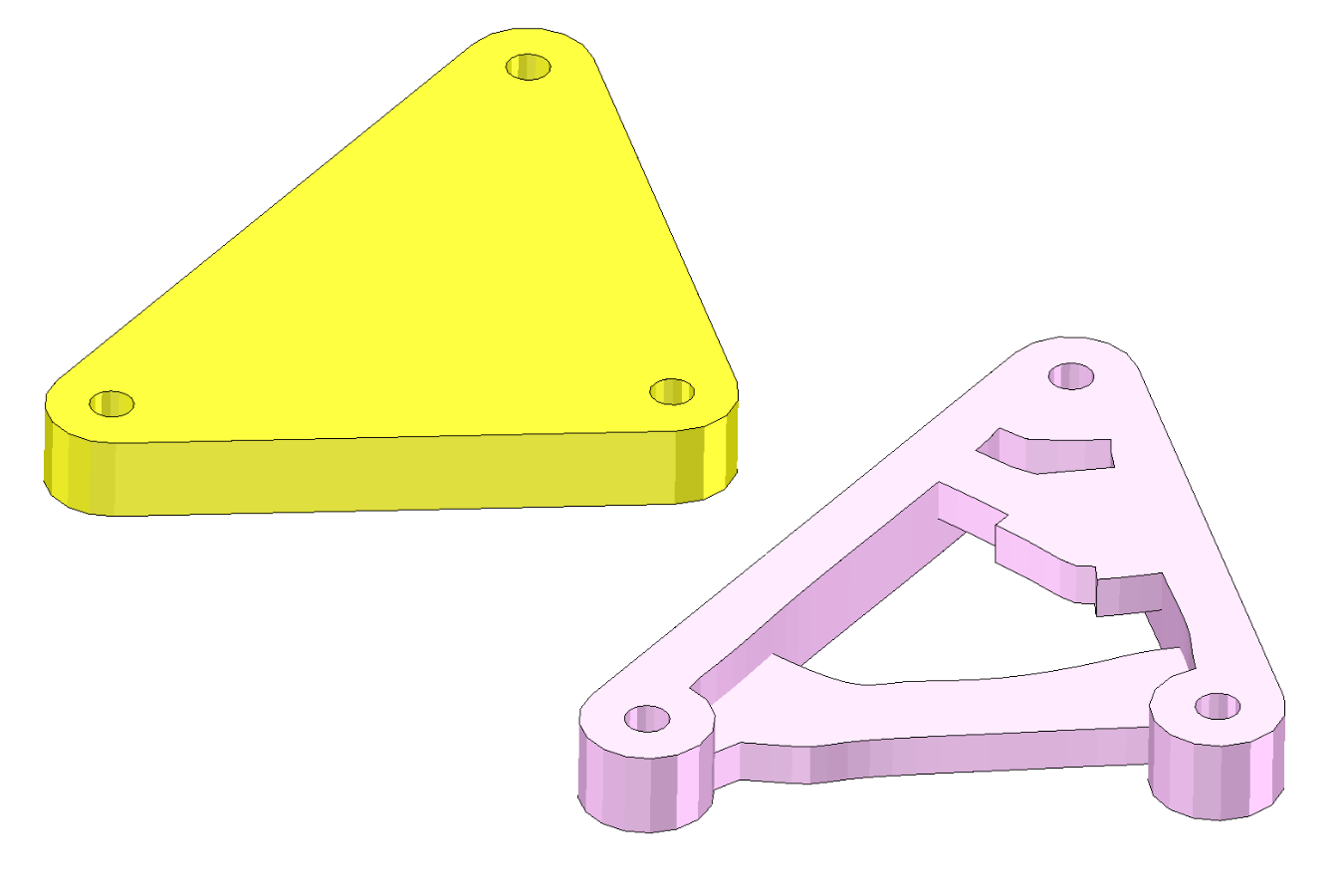 |
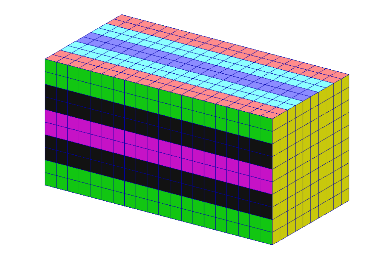
MSC Nastran Topology Optimization - Minimizing mass with stress and displacement constraints A solid block of material composed of 3D or Hexahedral elements is subjected to two load cases. Topology Optimization is used to minimize the mass of the structure, while satisfying both stress and displacement design constraints. Starting BDF Files: Link Solution BDF Files: Link |
Link | Link | Link |
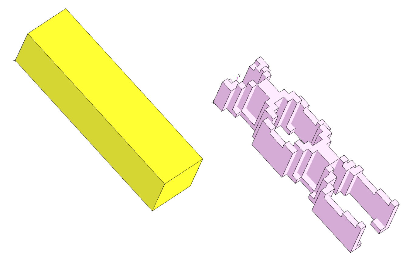 |
MSC Nastran Topology Optimization Manufacturing Constraints A cantilever beam is composed of 3D or Hexahedral elements and a load is applied at the free end. Topology Optimization is used to identify regions of material to remove. This example discusses options to produce a symmetric design and a design that can be manufactured via casting. Starting BDF Files: Link Solution BDF Files: Link |
Link | Link | Link |
 |
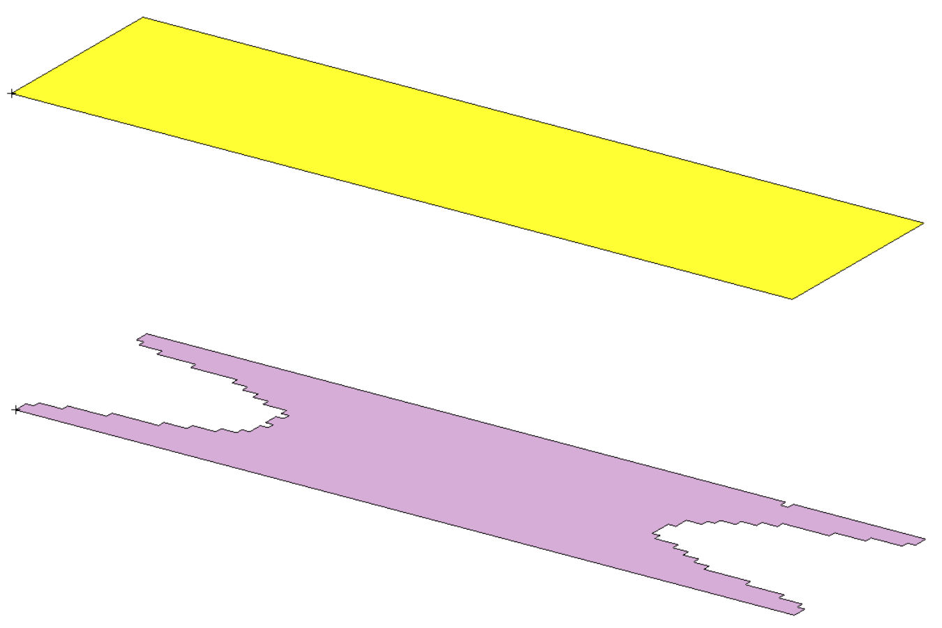
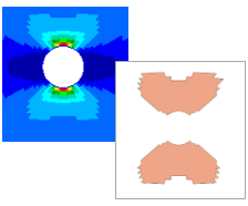
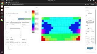
MSC Nastran Topology Optimization Mirror Symmetry Constraints A plate composed of 2D finite elements, is simply supported and has a load applied at the midpoint. Topology Optimization is used to identify material to remove. This example focuses on satisfying weight, stiffness and symmetry targets. Starting BDF Files: Link Solution BDF Files: Link |
Link | Link | Link |
 |
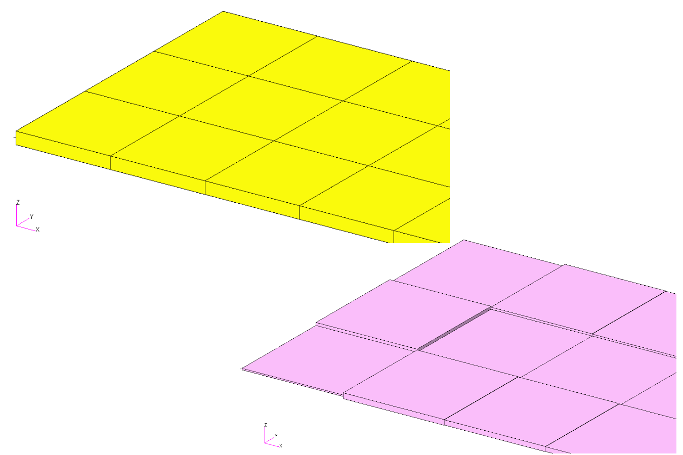
MSC Nastran Topology Optimization - Multidiscipline - Static Loading and Natural Frequency A simply supported plate is composed of 2D finite elements and a load is applied at the midspan. The MSC Nastran Topology Optimization capability is used to determine which portions of the plate should be kept while satisfying weight, stiffness and first natural frequency constraints. This example also showcases the ability to optimize for multiple analysis types, e.g. static and normal modes analysis. Starting BDF Files: Link Solution BDF Files: Link |
Link | Link | Link |
 |
MSC Nastran Topometry Optimization of a Cantilever Plate This tutorial is an introduction to Topometry Optimization. A simple cantilever plate is used to demonstrate element-by-element optimization of thickness. Starting BDF Files: Link Solution BDF Files: Link |
Link | Link | Link |
 |
MSC Nastran Topometry Optimization of a Composite Panel This tutorial covers the use of Topometry Optimization to determine ply shapes. Starting BDF Files: Link Solution BDF Files: Link |
Link | Link | |
 |
MSC Nastran Topometry Optimization with Symmetry Constraints This tutorial details the configuration of symmetry constraints in a topometry optimization. Starting BDF Files: Link Solution BDF Files: Link |
Link | ||
 |
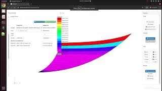
MSC Nastran Topography Optimization - Bead or Stamp Optimization This tutorial covers the use of Topography Optimization to determine optimal bead or stamp patterns. The Post-processor web app is used afterwards to review the results of the optimization. Starting BDF Files: Link Solution BDF Files: Link |
Link |
Advanced Optimization Tutorials
| Title and Description | PDF Tutorial | YouTube Tutorial |
|---|---|---|
| Manually Starting MSC Nastran and Uploading Results This tutorial discusses how to manually start MSC Nastran. This tutorial also discusses how to upload result files (.f06, .csv or multiopt.log) to the SOL 200 Web App. | Link | Link |
| CSV Export and Import for Design Variables, Responses and Constraints Large design models may have thousands of design variables and constraints. The web app supports the export and import of CSV files. With the aid of Excel, hundreds of entries can be rapidly configured. This tutorial discusses the CSV export and import functionality. | Link | |
| Responses in Design Model Responses are the outputs following a structural analysis. Some examples include displacements at nodes, stresses in elements, etc. Each design cycle during the optimization process involves a structural analysis and the production of responses. This tutorial discuses the use of the Responses App to carefully inspect responses found in the .f06 file. | Link | |
| The Design Cycle Process of MSC Nastran SOL 200/Optimization MSC Nastran Optimization or SOL 200 takes multiple design cycles to shift the design variable values, for example dimensions of your structure, until an optimum of your objective is reached. This video walks you through the design cycle process in MSC Nastran Optimization. |
Link | |
| Summary of Design Cycle History in the .f06 file - MSC Nastran Optimization At the end of an optimization with MSC Nastran, the final summary of the optimization is available at the bottom of the .f06 file. This video discusses how to interpret the final summary. |
Link | |
| Viewing Optimization results in Excel - MSC Nastran Optimization The results of an MSC Nastran Optimization can be viewed in excel. Information such as the change of objective and design variables can be viewed for each design cycle. This video walks you through the process of viewing optimization results in excel. |
Link | |
| How to create a new bdf file with optimized properties - MSC Nastran Optimization Once MSC Nastran Optimization has produced optimized design variables, e.g. optimized structural dimensions, the original .bdf/.dat file must be updated with the new property values. This video establishes two methods of updating the original .bdf/.dat file. |
Link | |
| How to fix 'RUN TERMINATED DUE TO HARD CONVERGENCE TO A BEST COMPROMISE INFEASIBLE DESIGN' MSC Nastran SOL 200 or Design Optimization employs an intelligent method of handling hundreds of design constraints. This video covers the following:
|
Link | |
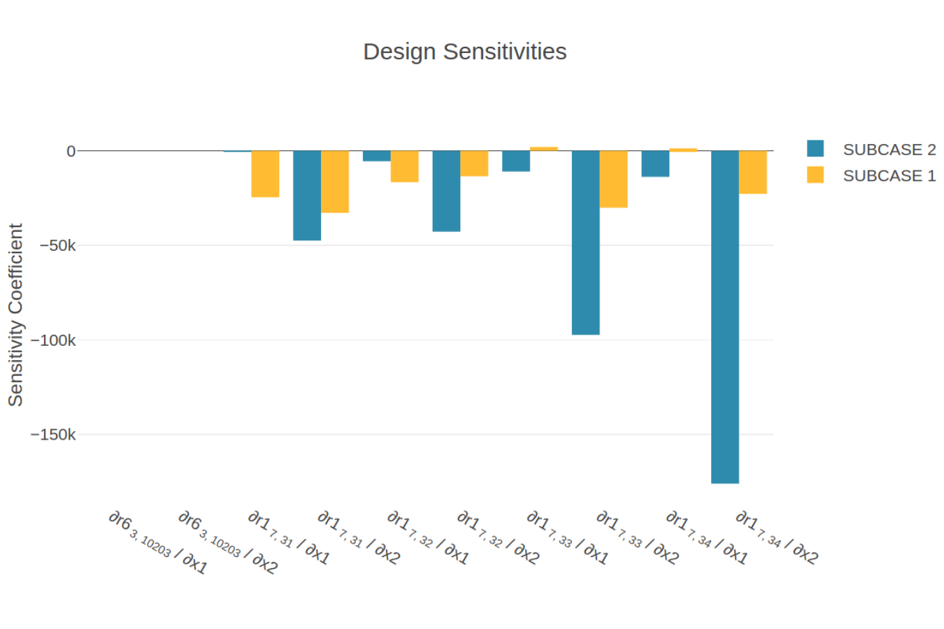
| How to perform a Sensitivity Analysis in MSC Nastran SOL 200 This video details 3 methods of performing a sensitivity analysis with MSC Nastran. The following points are discussed: What is sensitivity analysis? How to perform a sensitivity analysis with MSC Nastran Interpreting the sensitivities |
Link | |
| How to verify design variables - MSC Nastran Optimization Configuring a design model for MSC Nastran Optimization is a simple process, but care must be taken to ensure the configuration was properly done. This video details how to verify that design variables have been properly configured. |
Link | |
| How to verify design constraints - MSC Nastran Optimization A simulation of a Finite Element model can produce an overwhelming amount of output such as displacements, stresses, strain, etc. Design constraints are imposed on specific outputs. This video outlines a procedure to ensure the design constraints are applied to the correct responses such as displacements, stresses, strains, etc. |
Link |
Miscellaneous Tutorials
| Title and Description | PDF Tutorial | YouTube Tutorial | |
|---|---|---|---|
 |
Use the HDF5 Explorer to Create Plots Starting with MSC Nastran 2016, results can be outputted to the HDF5 file type. This tutorial introduces the HDF5 Explorer and the following concepts:
|
Link | |
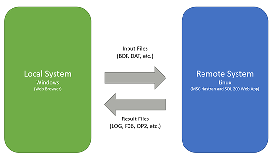 |
Remote execution of MSC Nastran on a remote operating system available on the local network This tutorial discusses the use of the Remote Execution web app and how to run MSC Nastran jobs on remote operating systems available on the local network. Traditionally, FTP and SSH programs are required to run MSC Nastran on remote operating systems, but this tutorial discusses how to run MSC Nastran through the web browser alone. FTP and SSH programs are not required for this tutorial. |
Link |
Machine Learning Tutorials
| Title and Description | PDF Tutorial | YouTube Tutorial | |
|---|---|---|---|
 |
Introduction - MSC Nastran Machine Learning Web App There are many machine learning methods available, such as neural networks, decision trees, genetic algorithms, supervised learning, etc. Watch this presentation to gain an understanding of the machine learning methods implemented in the MSC Nastran Machine Learning web app. The MSC Nastran Machine Learning web app makes use of the following methods:
|
Link | Link |
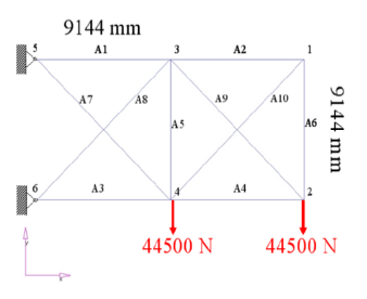 |
Machine Learning, Structural Optimization of a 10 Bar Truss with MSC Nastran SOL 400 Machine learning methods are used to optimize a truss structure. This example features the optimization of nonlinear responses from MSC Nastran SOL 400. MSC Nastran is used to evaluate the FE model. The design variables are the cross-sectional areas of the rod elements. The objective is to minimize the weight of the structure while constraining the axial stresses and displacements. Most machine learning examples are lower dimension problems with 1 to 5 parameters. This tutorial demonstrates a higher dimension scenario with 10 parameters. Starting Files: Link Solution BDF Files: Link |
Link | Link |
|
Machine Learning, Structural Optimization of a 3 Bar Truss Machine learning methods are used to optimize a truss structure. MSC Nastran is used to evaluate the FE model. The design variables are the cross-sectional areas of the rod elements. The objective is to minimize the weight of the structure while constraining the axial stresses. Starting Files: Link Solution BDF Files: Link |
Link | Link |
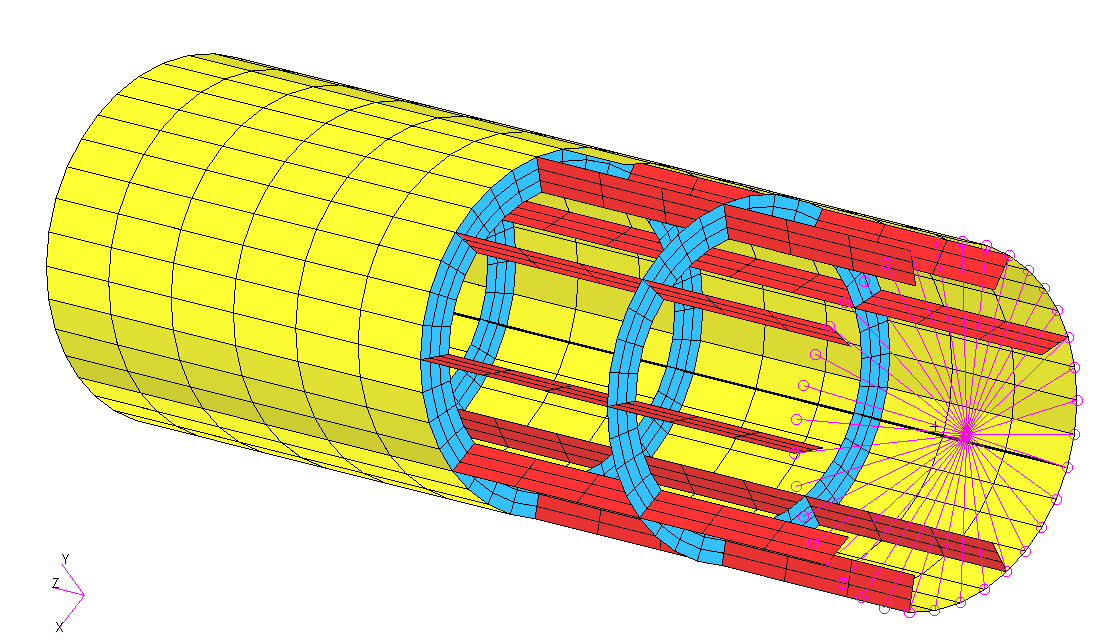 |
Machine Learning, Nonlinear Buckling (Post-Buckling) Optimization of a Reinforced Cylinder with MSC Nastran SOL 400 A reinforced cylinder is fixed at the base and a load is applied laterally at its top. Machine learning is performed to determine the optimal thicknesses of the reinforcements to achieve a minimum eigenvalue of 30 while minimizing the weight. This example features the optimization of nonlinear responses from MSC Nastran SOL 400 and involves nonlinear buckling (post-buckling) analysis. Starting Files: Link Solution BDF Files: Link |
Link | Link |
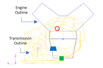 |
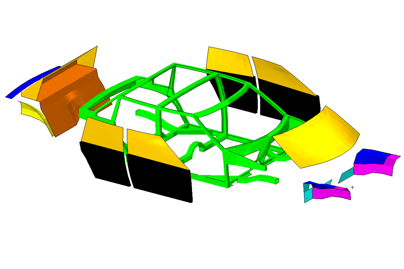
Parameter Study, Global Optimization with a Latin Hypercube Design Consider the optimization of a generic engine model that represents a V6 engine and automatic transmission as well as other components such as engine mount, transmission mount, crankshaft, drive axles, and flywheel. The Parameter Study web app is used to configure multiple local optimizations, each with different initial values for the variables, and MSC Nastran is used to perform each optimization. Frequency response plots are created afterward. The process of performing multiple local optimizations, then taking the best, or optimal, design is known as Global Optimization. Starting Files: Link Solution BDF Files: Link |
Link | Link |
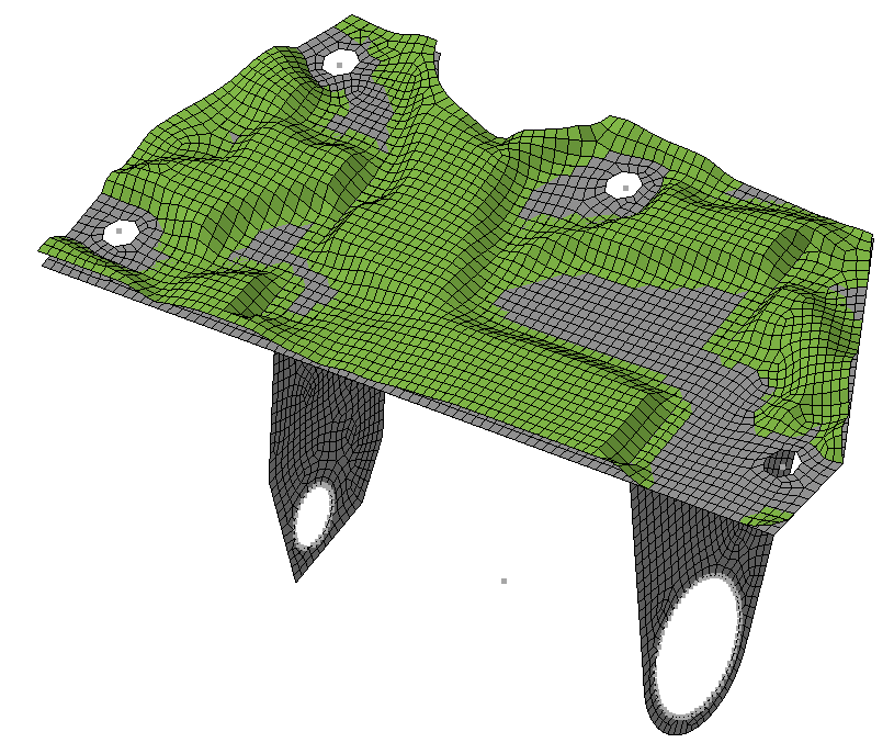
 |
Parameter Study, Varying the Location of Concentrated Masses A frequency response analysis is performed on a bracket. The goal in this tutorial is to vary the position of 5 concentrated masses on the bracket and determine the displacement vs. frequency plots for each different configuration of concentrated masses. In total, six MSC Nastran runs are configured, each with a different configuration of the concentrated masses. Starting Files: Link Solution BDF Files: Link |
Link | |
 |
Parameter Study, Varying the Position of Extra Supports The location of supports on a structural or mechanical system greatly influences its stiffness. This tutorial discusses one method to vary the location of supports and view displacement vs. frequency plots. Starting Files: Link Solution BDF Files: Link |
Link | |
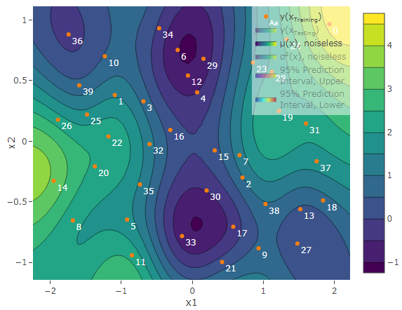 |
Prediction Analysis, Gaussian Process Regression This tutorial demonstrates the use of Gaussian process regression. |
Link | Link |
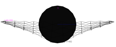 |
Prediction Analysis, Dynamic Impact of a Rigid Sphere on a Woven Fabric Consider a transient analysis of a rigid sphere impacting a woven fabric. The parameters allowed to vary include the friction coefficients. The response of interest are the displacements. This tutorial describes how to configure multiple MSC Nastran runs to generate training data. Gaussian process regression is used to train a surrogate model and make predictions. The prediction performance of the surrogate model is also evaluated. Also discussed are instructions to create displacement vs. time plots. Starting Files: Link Solution BDF Files: Link |
Link | |
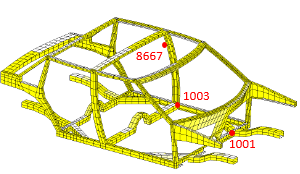 |
Prediction Analysis, Frequency Response Analysis (SOL 111) Consider a frequency response analysis of a ground vehicle. For different configurations of the ground vehicle, there is a desire to rapidly determine the frequency responses, including accelerations and pressures, while keeping the number of Finite Element (FE) solver runs to a minimum. This tutorial describes the procedure to use Gaussian progress regression as a surrogate model for computationally expensive Finite Element (FE) based simulations. This tutorial walks users through the process of acquiring training data, fitting the surrogate model, making predictions and quantifying uncertainty. In addition, the process to screen variables/parameters via Automatic relevance determination (ARD) is discussed. Starting Files: Link Solution BDF Files: Link |
Link | |
 |
Prediction Analysis, Buckling Consider a linear buckling analysis. The parameter allowed to vary is a spring constant. The response of interest is the buckling load factor. This tutorial describes how to configure multiple MSC Nastran runs to generate training data. Gaussian process regression is used to train a surrogate model and make predictions. The prediction performance of the surrogate model is also evaluated. Starting Files: Link Solution BDF Files: Link |
Link | |
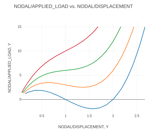 |
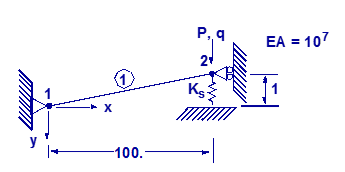
Prediction Analysis, Post-Buckling Consider a post-buckling analysis. The parameter allowed to vary is a spring constant. The responses of interest include the applied load and displacements. This tutorial is similar to the previous tutorial named Prediction Analysis, Buckling. Like the previous tutorial, this tutorial discusses the use of Gaussian process (GP) regression to train a surrogate model. To expand your experience with GP regression, this tutorial purposely demonstrates a scenario where a poorly fitted model is obtained and what the procedure is to remedy this issue. Also discussed are instructions to create load vs. displacement plots . Starting Files: Link Solution BDF Files: Link |
Link |
Beams Tutorials
| Title and Description | PDF Tutorial | YouTube Tutorial | |
|---|---|---|---|
 |
Introduction to the PBMSECT Web App This introductory tutorial details the use of the PBMSECT web app to generate arbitrary beam cross sections. The PBMSECT web app is used to automatically generate and manage the following bulk data entries: PBMSECT, PBRSECT, POINT and SET1. |
Link | Link |
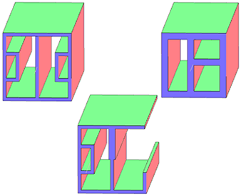 |
Examples of arbitrary beam cross sections with PBMSECT and PBRSECT This tutorial describes the procedure to generate different types of arbitrary beam cross sections, including open or closed profiles. Starting BDF Files: Link Solution BDF Files: Link |
Link | Link |
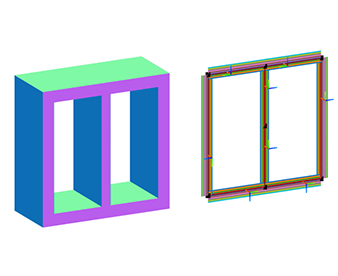 |
Composite Arbitrary Beam Cross Section Composite arbitrary beam cross section (ABCS) may be defined through the use of the PBMSECT and CBEAM3 entries. This tutorial details the use of the PBMSECT web app to construct a composite ABCS and generate the necessary PBMSECT, POINT and SET1 entries. Important considerations, such as ply coordinate systems and validating the FEM of the beam cross section, are discussed. Starting BDF Files: Link Solution BDF Files: Link |
Link | Link |
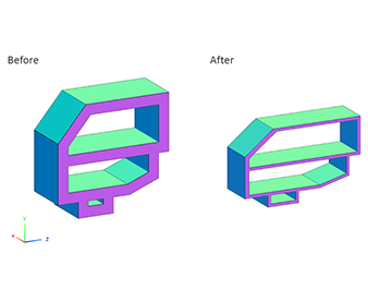 |
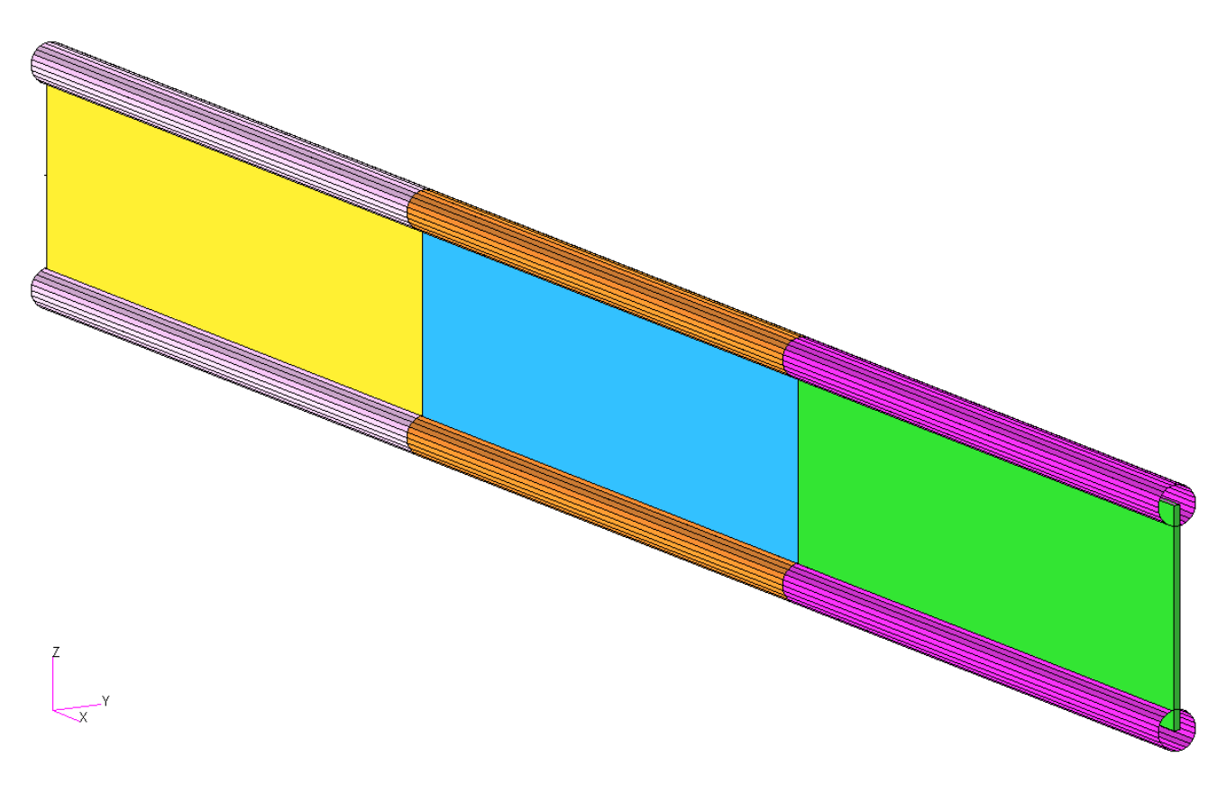
Arbitrary Beam Cross Section Optimization MSC Nastran SOL 200 supports varying the width, height and wall thickness of arbitrary beam cross sections (ABCS) defined by the PBRSECT or PBMSECT entries. This tutorial walks you through the process of generating an ABCS via the PBMSECT entry, configuring an optimization for MSC Nastran SOL 200, and reviewing the optimization results. Starting BDF Files: Link Solution BDF Files: Link |
Link | Link |
Composite Laminate Optimization Tutorials
| Title and Description | PDF Tutorial | YouTube Tutorial | |
|---|---|---|---|
 |
Composite Coupon – Phase A – Determination of the optimal 0° direction of a composite The goal of this 5-phase tutorial series is to optimize a composite coupon, with a core, and produce a lightweight composite that satisfies failure index constraints. The optimal ply shapes (ply drop-offs) and ply numbers are determined for 0°, ±45°, and 90° plies. A stacking sequence optimization is performed to satisfy manufacturing requirements. One important part of optimizing composites is visualizing the composite plies. This tutorial series also demonstrates the visualization of ply drop-offs, tapered plies and core layers. This first phase involves determining the optimal 0° direction of a composite. It is best practice to align the 0° plies in the direction of the load. Not doing so will more than likely produce a suboptimal composite that is heavier than necessary. This tutorial demonstrates the use of MSC Nastran's optimizer to determine the optimal 0° direction of a composite. An optimization is performed to maximize the stiffness of the composite for multiple load cases and while varying the angle of the 0° plies. Ultimately, the best 0° direction is determined. This is the first phase in a 5-phase tutorial series. Starting BDF Files: Link Solution BDF Files: Link |
Link | Link |
|
Composite Coupon – Phase B – Baseline Ply Number Optimization This tutorial demonstrates how to configure a basic ply number optimization of continuous plies that span the entire model. The goal of this tutorial is to demonstrate basic actions such as creating variables, a weight objective and constraints on failure index. The results of this ply number optimization serve as a baseline for future comparisons. In a subsequent tutorial, the ply shapes will be optimized to minimize weight. This is the second phase in a 5-phase tutorial series. Starting BDF Files: Link Solution BDF Files: Link |
Link | Link |
 |
Composite Coupon – Phase C – Data Preparation for Ply Shape Optimization This tutorial is a guide to preparing data for ply shape optimization in a subsequent tutorial. The maximum failure index values of the outer plies of the composite are determined and saved to specially formatted PLY000i files. The PLY000i files will be used to construct optimal ply shapes in a subsequent tutorial. This is the third phase in a 5-phase tutorial series. Starting BDF Files: Link Solution BDF Files: Link |
Link | Link |
 |
Composite Coupon – Phase D – Ply Shape and Ply Number Optimization This tutorial details the process to build optimal ply shapes and perform a ply number optimization. The optimal ply shapes are constructed to follow the contours of the failure indices. The ply number optimization involves minimizing weight and constraining the failure indices of plies. The PLY000i files and BDF files from the previous tutorial, phase C, are used in this tutorial. This is the fourth phase in a 5-phase tutorial series. Starting BDF Files: Link Solution BDF Files: Link |
Link | Link |
 |
Composite Coupon – Phase E – Stacking Sequence Optimization This tutorial involves performing a stacking sequence optimization and is a continuation of the previous tutorial, phase D. A final statics analysis is performed to confirm the optimized composite satisfies failure index constraints. This is the fifth phase in a 5-phase tutorial series. Starting BDF Files: Link Solution BDF Files: Link |
Link | Link |
| Title and Description | PDF Tutorial | YouTube Tutorial | |
|---|---|---|---|
 |
Sandwich Composite Panel – Phase B – Baseline Core Thickness Optimization The goal of this 3-phase tutorial series is to optimize a curved composite panel, with a core, and produce a lightweight composite that satisfies constraints on the buckling load factor. This tutorial series focuses exclusively on optimizing the thickness of the core. The methods detailed in the tutorial series are applicable to both foam and honeycomb cores. This tutorial demonstrates how to configure a basic core thickness optimization where the core has a constant thickness throughout the entire model. The goal of this tutorial is to demonstrate basic actions such as creating variables, a weight objective and constraints on the buckling load factor. The results of this core thickness optimization serve as a baseline for future comparisons. In a subsequent tutorial, the core will be allowed to have a variable thickness throughout the model and will be optimized to minimize weight. This is the first phase in a 3-phase tutorial series. Starting BDF Files: Link Solution BDF Files: Link |
Link | Link |
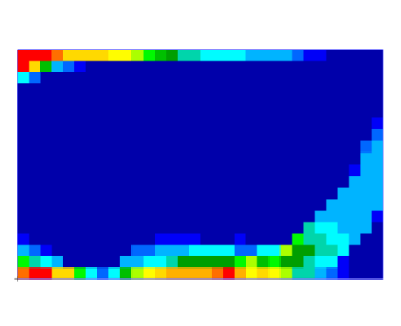 |
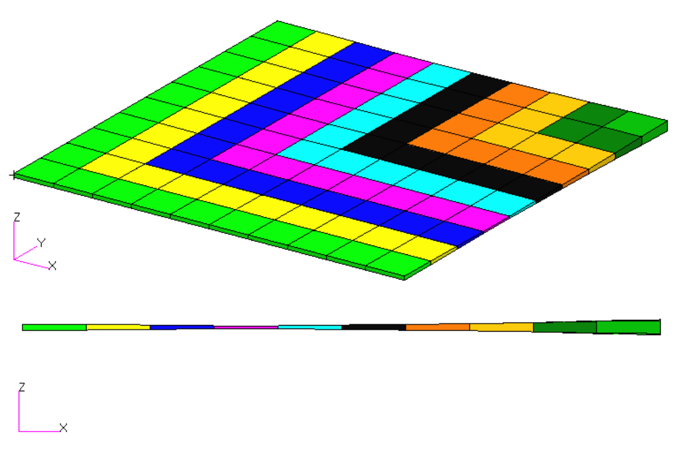
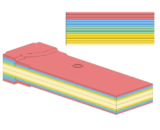
Sandwich Composite Panel – Phase C – Topometry Optimization to Determine Optimal Core Shape This tutorial is a guide to preparing data for core shape and core thickness optimization in a subsequent tutorial. A topometry optimization is performed in this tutorial to determine the ideal thickness distribution of the core throughout the entire composite panel while satisfying constraints on the buckling load factor and minimizing weight. The results of a topometry optimization are contained in the PLY000i files and will be used to construct optimal core shapes in a subsequent tutorial. This is the second phase in a 3-phase tutorial series. Starting BDF Files: Link Solution BDF Files: Link |
Link | Link |
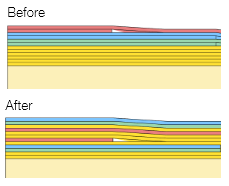
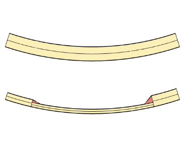 |
Sandwich Composite Panel – Phase D – Core Shape and Core Thickness Optimization This tutorial details the process to build optimal core shapes and perform a core thickness optimization. The optimal core shapes are constructed to follow the contours of thickness results generated by a topometry optimization. The core thickness optimization involves minimizing weight and constraining the buckling load factor. The PLY000i files and BDF files from the previous tutorial, phase C, are used in this tutorial. Comparisons are made between this optimization in phase D and the baseline optimization performed in phase B. This is the third phase in a 3-phase tutorial series. Starting BDF Files: Link Solution BDF Files: Link |
Link | Link |
Shape Optimization Tutorials
| Title and Description | PDF Tutorial | YouTube Tutorial | |
|---|---|---|---|
 |
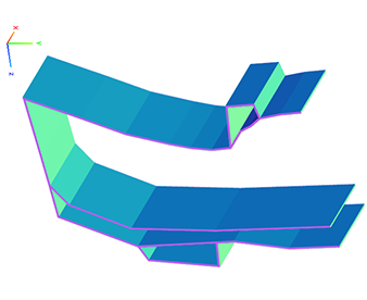
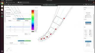
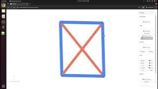
Shape Optimization of a Cantilever Beam This tutorial is an introduction to MSC Nastran's Shape Optimization capability. A cantilever beam is configured for a shape optimization. The goal is to minimize the mass while satisfying stress constraints. Specified regions of the beam are allowed to expand or contract and define the shapes that will vary during the optimization. This tutorial discusses the following concepts: auxiliary models, shape basis vectors, scaling shape basis vectors, configuring variable bounds, strategies to prevent mesh distortions, results interpretation, updating the model, and more. Starting BDF Files: Link Solution BDF Files: Link |
Link | Link |
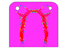
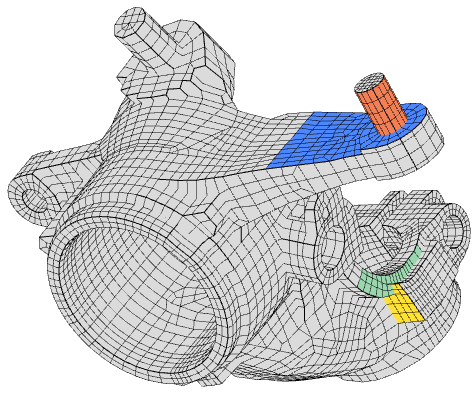 |
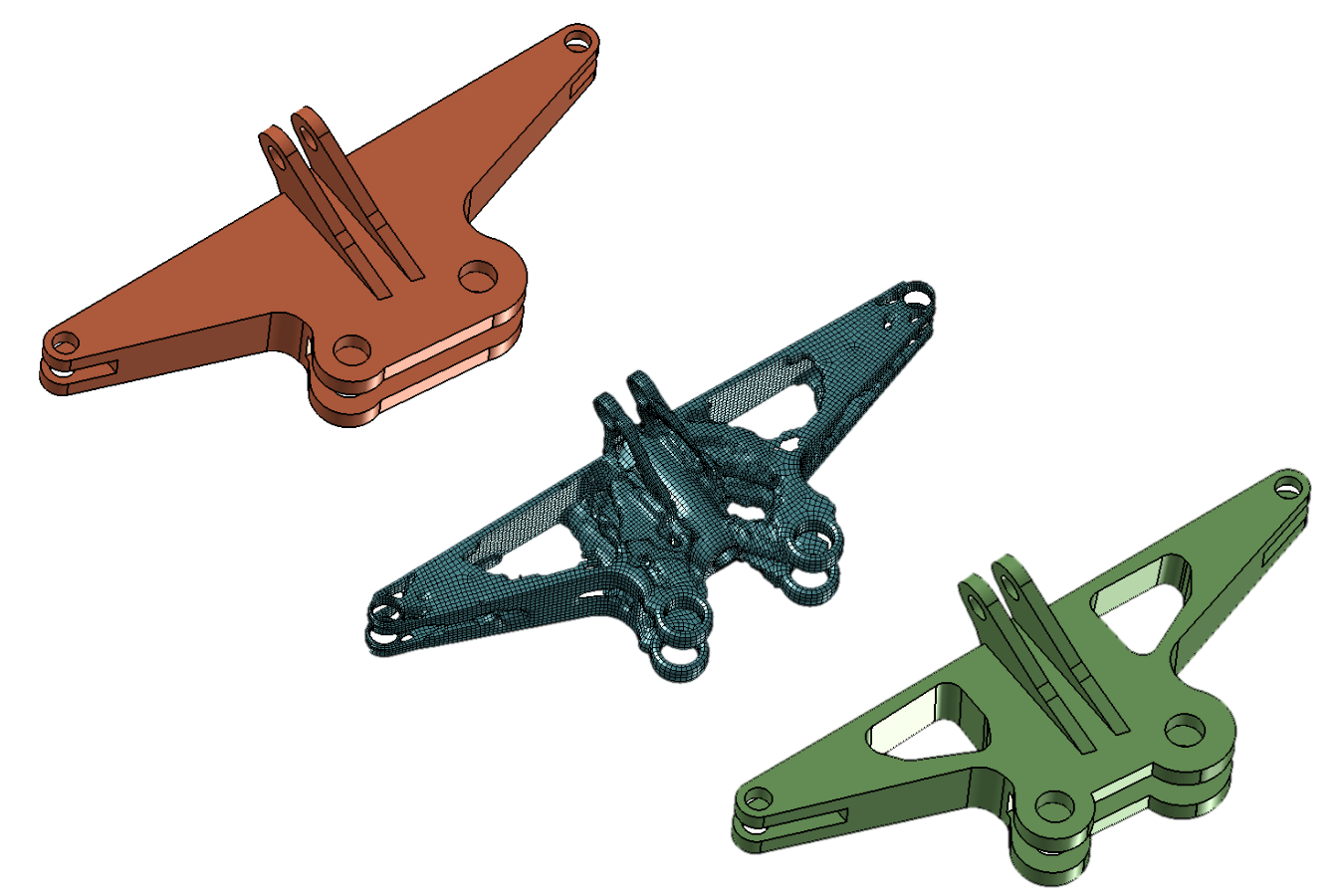
Shape Optimization of a Steering Knuckle A steering knuckle is configured for a shape optimization. The goal is to minimize the mass while satisfying stress constraints. Twelve load cases are considered. Four regions of the model are allowed to expand or contract and define the shapes that will vary during the optimization. This tutorial is an advanced shape optimization tutorial and utilizes MSC Nastran's shape optimization capability. Starting BDF Files: Link Solution BDF Files: Link |
Link | Link |
Post-processor Tutorials
| Title and Description | PDF Tutorial | YouTube Tutorial | |
|---|---|---|---|
 |
MSC Nastran Results - Introduction to Nastran Results - Displacements, forces, stresses and composite ply stresses for entries CQUAD4, CTRIA3, CQUAD8, CBEAM, CBUSH, CFAST, PSHELL, PCOMP, PBMSECT, PBUSH and PFAST
This tutorial is an introduction to Nastran results.
Starting BDF Files: Link |
Link | Link |
 |
MSC Nastran Results - CBAR - Element forces, stresses and displacements
The goal of this exercise is to review the results from a statics analysis. The element forces, bending stresses, displacements and twist of CBAR elements is displayed. Source of Exercise Problem 1: Linear Statics, Rigid Frame Analysis Patran Reference Manual, Part 6: Results Postprocessing, Chapter 15 - Verification and Validation Starting BDF Files: Link |
Link | |
 |
MSC Nastran Results - PCOMP - Ply stresses
The goal of this exercise is to view the ply stresses of a 3 layer composite laminate. Source of Exercise Problem 2: Linear Statics, Cross-Ply Composite Plate Analysis Patran Reference Manual, Part 6: Results Postprocessing, Chapter 15 - Verification and Validation Starting BDF Files: Link |
Link | |
 |
MSC Nastran Results - CQUAD4 - Stresses and deformations in spherical coordinates
The goal of this exercise is to inspect the deformation and stresses of an FE model configured in the spherical coordinate system. Source of Exercise Problem 5: Linear Statics, 2D Shells in Spherical Coordinates Patran Reference Manual, Part 6: Results Postprocessing, Chapter 15 - Verification and Validation Starting BDF Files: Link |
Link | |
 |
MSC Nastran Results - CROD - Axial forces and stresses
The goal of this exercise is to plot the deformations, axial forces and stresses of CROD elements. Source of Exercise Problem 8: Linear Statics, Pinned Truss Analysis Patran Reference Manual, Part 6: Results Postprocessing, Chapter 15 - Verification and Validation Starting BDF Files: Link |
Link | |
 |
MSC Nastran Results - CGAP - Element force and stresses in CGAP elements
The goal of this exercise is to inspect the element forces and displacements in CGAP elements. Source of Exercise Problem 13: Nonlinear Statics, Beams with Gap Elements Patran Reference Manual, Part 6: Results Postprocessing, Chapter 15 - Verification and Validation Starting BDF Files: Link |
Link | |
 |
MSC Nastran Results - CONM2 and CELAS1 - Natural Frequencies, Mode Shapes, Spring Mass
The goal of this exercise is to inspect the natural frequencies and mode shapes of a spring mass system. Source of Exercise Problem 14: Normal Modes, Point Masses and Linear Springs Patran Reference Manual, Part 6: Results Postprocessing, Chapter 15 - Verification and Validation Starting BDF Files: Link |
Link | |
 |
MSC Nastran Results - CTRIA - Natural Frequencies, Mode Shapes, Cylindrical Coordinates
The goal of this exercise is to inspect the natural frequencies and mode shapes of an FE model composed of CTRIA elements. Source of Exercise Problem 16: Normal Modes, Pshells and Cylindrical Coordinates Patran Reference Manual, Part 6: Results Postprocessing, Chapter 15 - Verification and Validation Starting BDF Files: Link |
Link | |
 |
MSC Nastran Results - Buckling Load Factor of a Thin Walled Cylinder
The goal of this exercise is to determine the eigenvalue from a buckling analysis and determine the buckling load. Source of Exercise Problem 17: Buckling, shells and Cylindrical Coordinates Patran Reference Manual, Part 6: Results Postprocessing, Chapter 15 - Verification and Validation Starting BDF Files: Link |
Link | |
 |
MSC Nastran Results - CHEXA - Transient Analysis in Cylindrical Coordinates
The goal of this exercise is to view the displacements of a static and transient analysis. The process to create displacement vs. time plots is also demonstrated. Source of Exercise Problem 19: Direct Transient Response, Solids and Cylindrical Coordinates Patran Reference Manual, Part 6: Results Postprocessing, Chapter 15 - Verification and Validation Starting BDF Files: Link |
Link | |
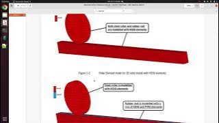 |
MSC Nastran SOL 400 Results - Displacements, forces of a steel roller moving on rubber
The displacements are displayed for a steel roller moving on a rubber base. Special consideration is given to the steel roller. A load vs. displacement plot is created for the steel roller. Source of Exercise Chapter 5: Steel Roller on Rubber MSC Nastran 2023.3 Demonstration Problems Manual - Implicit Nonlinear Starting BDF Files: Link |
Link | |
 |
MSC Nastran SOL 400 Results - CBUSH,CFAST,CWELD - Shear Forces in Fasteners of a Lap Joint
The shear forces in fasteners of a lap joint are displayed. The fasteners are modeled with CBUSH, CFAST and CWELD elements. Source of Exercise Chapter 33: Large Rotation Analysis of a Riveted Lap Joint MSC Nastran 2023.3 Demonstration Problems Manual - Implicit Nonlinear Starting BDF Files: Link |
Link | |
 |
MSC Nastran SOL 400 Results - Load vs. Deflection Graph (Load Stroke Plot)
This exercise the procedure to create load vs. deflection graphs, also known as load stroke plots. Source of Exercise Chapter 36: Shallow Cylindrical Shell Snap-through MSC Nastran 2023.3 Demonstration Problems Manual - Implicit Nonlinear Starting BDF Files: Link |
Link |
Uncertainty Quantification
| Title and Description | PDF Tutorial | YouTube Tutorial | |
|---|---|---|---|
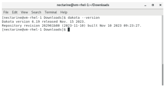 |
Uncertainty Quantification - Installing Sandia Dakota on Windows and Red Hat Linux 7 This tutorial details the process to download and configure Sandia Dakota on Windows and Red Hat Linux 7. |
Link | |
 |
Uncertainty Quantification - 10 Bar Truss with MSC Nastran This example details the use of uncertainty quantification to reduce the variability of responses when uncertain parameters are present. Forward propagation of uncertainty is the focus of this exercise and the sampling method is used for uncertainty quantification. A 10 bar truss with 4 uncertain parameters is considered and a Latin Hypercube sampling is used. The quantities of interest include the mean and standard deviation values of the responses and correlation coefficients between the inputs (parameters) and outputs (responses). Starting BDF Files: Link Solution BDF Files: Link |
Link |
Optimization Under Uncertainty
| Title and Description | PDF Tutorial | YouTube Tutorial | |
|---|---|---|---|
 |
Optimization Under Uncertainty - 3 Bar Truss, Part 1 of 2 There are many methods available for uncertainty quantification to approximate statistics such as mean, standard deviation and tail probabilities of stochastic responses. Each method has its own computational cost. During an optimization under uncertainty (OUU), an uncertainty quantification (UQ) is performed frequently. If the cost of each UQ is high, the OUU’s computational costs will also be prohibitively high. The mean value first-order second-moment (MVFOSM) method is one of the least expensive UQ methods and involves one black box function evaluation to acquire the response values and gradients. From a single evaluation, the required statistics are approximated, and is a contrast to other UQ methods that may require dozens or hundreds of black box function runs. The MVFOSM is limited to responses that are linear and normally (Gaussian) distributed and is not universally appropriate. This exercise details a procedure to determine if the MVFOSM method is appropriate to approximate the statistics of stress responses of a 3-bar truss. If the MVFOSM is suitable, this will significantly reduce the number of black box function runs necessary to perform the UQ and OUU. The black box function is the FEA solver MSC Nastran. MSC Nastran is used to perform the finite element analysis and acquire responses and gradients. Sandia Dakota is used to perform the UQ. The SOL 200 Web App is used to configure the UQ. This is part 1 of a 2-part tutorial. Starting BDF Files: Link Solution BDF Files: Link |
Link | Link |
 |
Optimization Under Uncertainty - 3 Bar Truss, Part 2 of 2 This example details the process to configure and perform an optimization under uncertainty (OUU) for a 3-bar truss. Also, details are included regarding how to interpret the OUU results and final probabilities of failure. The uncertainty quantification (UQ) is performed via the mean value first-order second-moment (MVFOSM) method. This is part 2 of a 2-part tutorial. The optimization problem statement is to minimize the mean mass while ensuring the stress constraints have a probability of failure no greater than 5%. MSC Nastran is used to perform the finite element analysis and acquire responses and gradients. Sandia Dakota is used to perform the UQ and OUU. The SOL 200 Web App is used to configure the OUU and will automatically exchange responses and gradients between MSC Nastran and Sandia Dakota. Starting BDF Files: Link Solution BDF Files: Link |
Link | Link |
 |
Optimization Under Uncertainty - 53 Bar Truss Both uncertainty quantification (UQ) and optimization under uncertainty (OUU) may require hundreds or thousands of black box function evaluations when considering a large number of uncertain variables. Certain black box functions will require hours or days for a single run, so thousands of black box function evaluations are impractical. Finite element solvers are such black box functions where at most a few hundred runs are practical. This tutorial details how to configure an OUU when a large number of uncertain variables are considered, and strategies are discussed to minimize the number of black box function runs. The OUU involves minimizing the mass of a 53-bar truss, varying the mean cross section area of 53 truss members (53 variables), and constraining the probability of failure to 5%, where failure occurs if the axial stress exceeds the material yield strength. This OUU may require 200 to 2000 black box function runs, so the strategies discussed are critical to reduce the number of runs necessary to converge to a solution. The black box function is the FEA solver MSC Nastran. MSC Nastran is used to perform the finite element analysis and acquire responses and gradients. Sandia Dakota is used to perform the UQ and OUU. The SOL 200 Web App is used to configure the OUU. Starting BDF Files: Link Solution BDF Files: Link |
Link | Link |
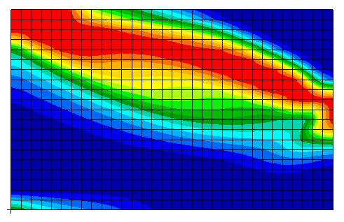
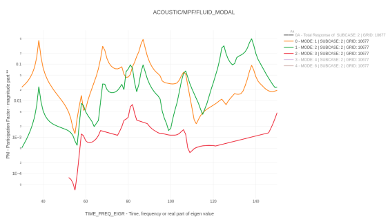
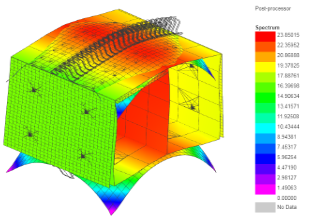
 |
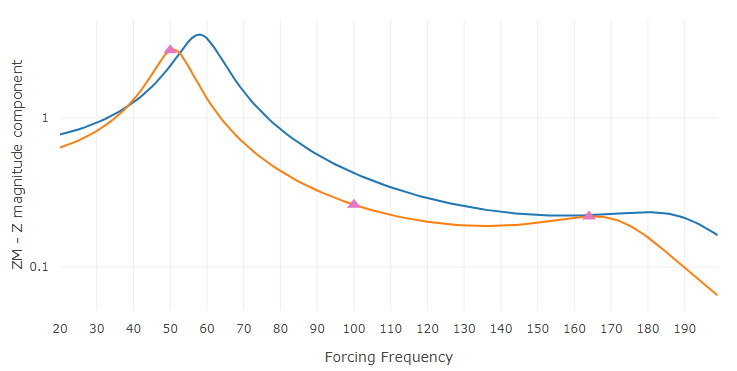
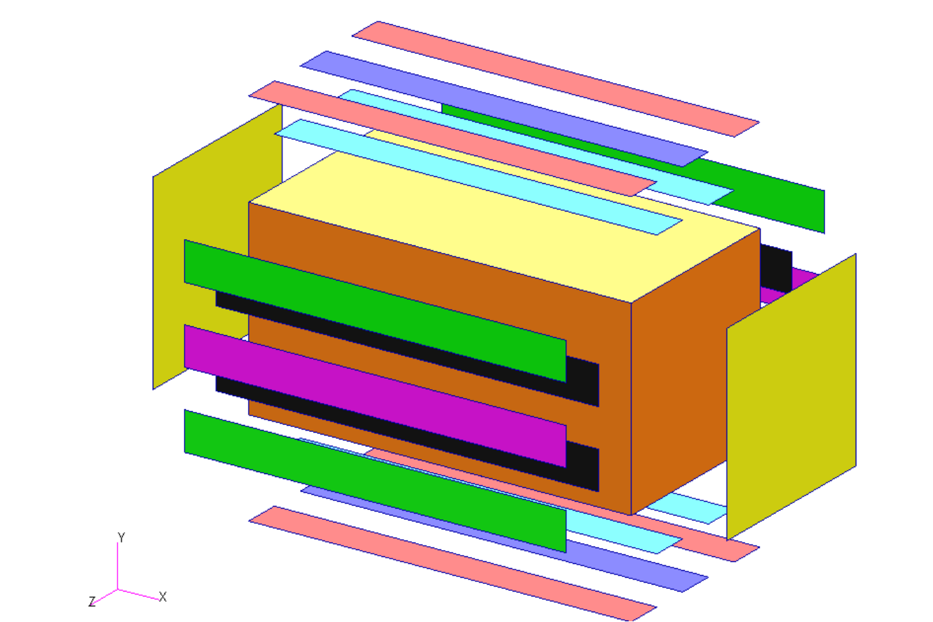
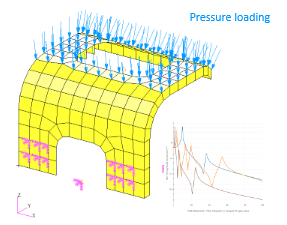
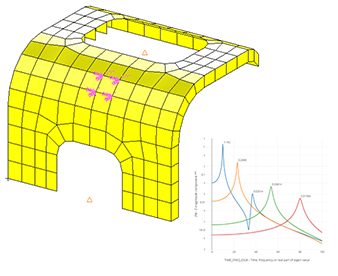
Robust Design Optimization - Acoustic Box Small deviations to structural or mechanical systems during manufacturing can result in significantly varying performance. Examples of varying performance include variations in hole diameters that can lead to variations in peak stress, and variations in gauge thicknesses that can lead to variations in acoustic peak pressures. This tutorial details the use of robust design optimization to reduce the variability of performance when input uncertainties are considered. Specifically, a robust design optimization is configured and performed to minimize the variability of responses. A finite element model is considered of an acoustic box subjected to a dynamic load. The uncertain variables correspond to the gauge thicknesses of the acoustic box. The robust design objective is to minimize the sum of mean and 3-standard deviations of peak acoustic pressures at 2 locations of the FE model. A constraint on mean mass is imposed. The FE solver MSC Nastran is used to perform the acoustic analysis and acquire the necessary responses. Sandia Dakota is used to perform the uncertainty quantification and robust design optimization. The SOL 200 Web App is used to configure both the uncertainty quantification and robust design optimization. Starting BDF Files: Link Solution BDF Files: Link |
Link | Link |
Presentations
| Title and Description | PDF Tutorial | YouTube Tutorial | |
|---|---|---|---|
|
Introduction to Nastran SOL 200 Design Sensitivity and Optimization This presentation introduces engineers to MSC Nastran's optimization capability known as SOL 200. The following topics are discussed:
|
Link | Link |
|
Introduction - MSC Nastran Machine Learning Web App There are many machine learning methods available, such as neural networks, decision trees, genetic algorithms, supervised learning, etc. Watch this presentation to gain an understanding of the machine learning methods implemented in the MSC Nastran Machine Learning web app. The MSC Nastran Machine Learning web app makes use of the following methods:
|
Link | Link |
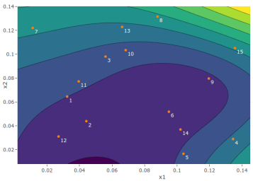 |
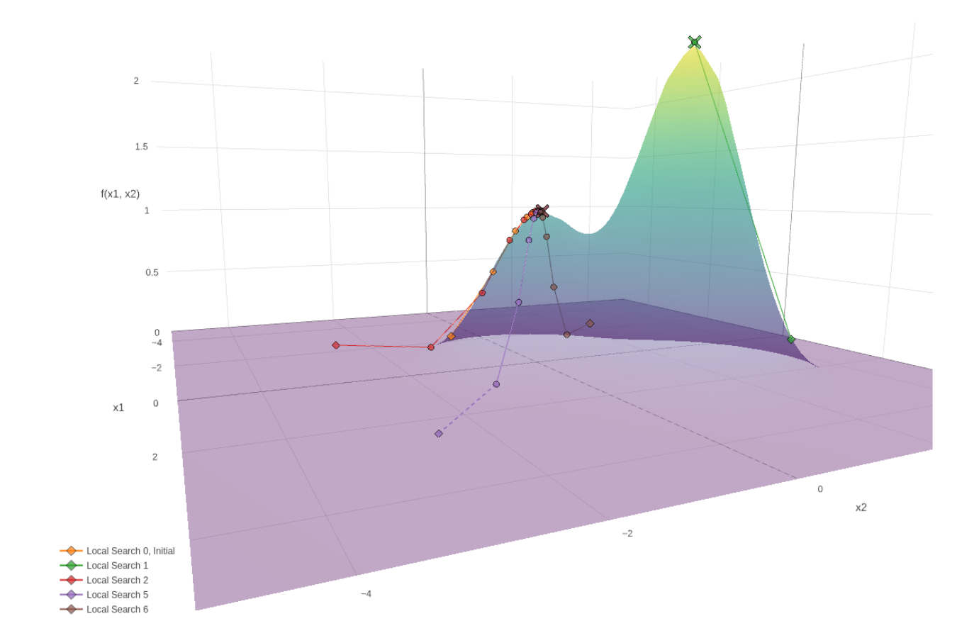
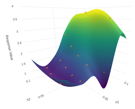
Shape Optimization of FEA Models by Machine Learning-Based Surrogate Modeling Some FEA solvers feature an embedded optimizer with shape optimization capabilities that expect users to specify the allowable movement of nodes on the mesh. This approach has proven effective for a small set of engineering problems but in most applications, during the optimization a mesh distortion occurs. There is an alternative to shape optimization that is not limited by mesh distortions. This presentation details the use of Gaussian process regression (GPR) to perform a simple shape optimization. While this presentation demonstrates a 2-parameter example, GPR is effective for shape optimization problems up to 10-parameters. |
Link | |
 |
Introduction to MSC Nastran Results This presentation is for new MSC Nastran users and discusses how to interpret MSC Nastran results. |
Link |